An Excel gridline is the faint gray edge around each cell in the worksheet. In addition to making it easier to read the data, these gridlines help distinguish between the cells. Unlike borders, where you can change color, width, style, etc., gridlines offer limited options for changing their appearance. In this article, you will learn 4 effective ways to change gridlines in Excel.
How to Change Gridlines in Excel: 4 Suitable Ways
1. Change Excel Gridlines Color
The default color for gridlines in worksheets is Automatic. Use the following procedure to change gridlines’ color.
1.1 Using Excel Advanced Options
Follow the steps below to use this technique.
Steps:
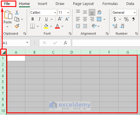
- First, make sure you’re selecting the worksheets for which you’d like to change the gridlines’ color. Then, go to the File tab.
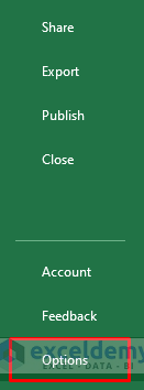
- Now, under the File tab, select Options.
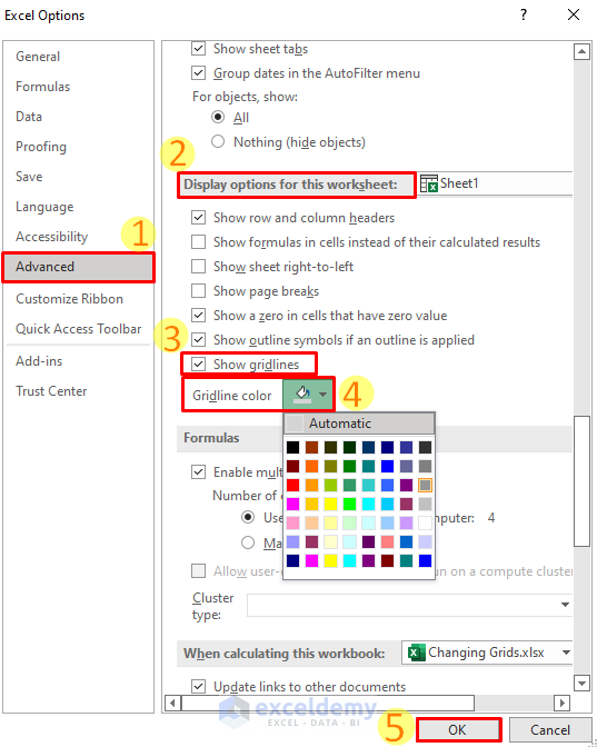
- Ensure that Show gridlines are selected in the Advanced category of this worksheet’s Display options.
- Click the color you want in the Gridline color box
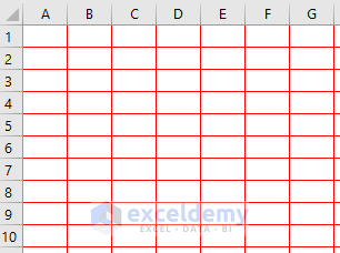
If you choose red, here is the output.
Note:
You can return gridlines to their default color by clicking Automatic.
1.2 Using Borders Option
This option allows you to color gridlines in your spreadsheet with any of the standard colors or your own custom color, such as a brand color. Just follow the steps below to do so.
Steps:
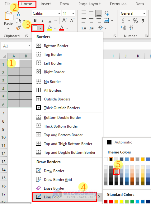
- The first step is to select the entire spreadsheet. Click the triangle on the top left corner of your spreadsheet or use Ctrl+A.
- Click on the Borders icon in your Home tab once your sheet is selected. Choose a color from the options under Line Color.
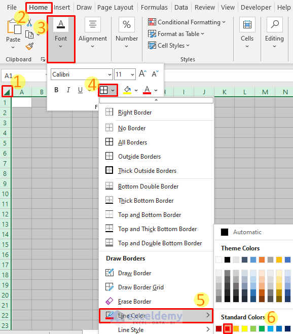
By pressing the Gridlines button again, you can change the style of your grid lines by selecting Line Style and selecting the type of line you’d like.
- Last but not least, select the Borders icon again and set it to All Borders.
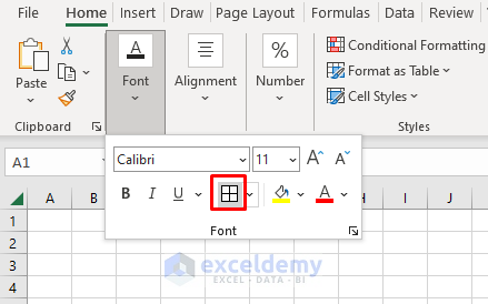
You’ll now see a new color on your Gridlines!

2. Change Height and Width of Gridlines
By using gridlines, you can align shapes and ensure that each object has the same dimensions. A gridline in Excel is simulated by a column border, and the width and height of each column basically determine the width and height of the gridline.
It is possible to change the gridline width for your worksheet if you wish. Just follow the steps below to do so.
Steps:
- To select all cells in the workbook, click on the top left corner

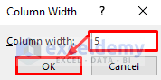
- Select Column Width by right-clicking on any column. A Column Width dialog box will pop up.

- Click OK after entering the new width value in the dialog box.
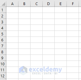
Here are the gridlines with new widths.
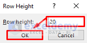
Similarly, you can change the height of the gridlines. To do so, just select Row Height by right-clicking on any row. A Row Height dialog box will pop up.
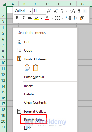
Finally, click OK after putting the new height value in the dialog box.
3. Show Gridlines for Specific Region
There are two options in Excel regarding the gridline: you can either display it throughout the entire worksheet or hide it completely. It is not possible to display this in a specific area.
In specific areas of the worksheet, borders can be used to create a gridline effect. There are many options for borders, and you can make them look exactly like gridlines (by choosing a light gray color).
Follow the steps below to do so.
Steps:
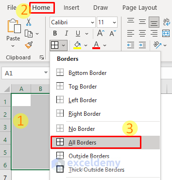
- First, select the region. Then, go to the Home tab >> Font group >> select All Borders from the Borders drop-down list.
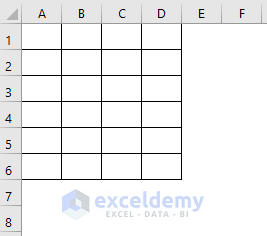
Here is the border acting as gridlines. Now we need to change the color of the borderline to the color of the original gridlines.
Select the specific borderline area. Go to the Home tab >> Font group >> select Line Color from the Draw Borders drop-down list. Now choose the gray color like as original gridline color.
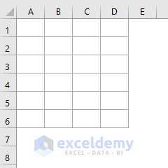
Finally, here are the gridlines for a specific region.
4. Remove Gridlines from Worksheet
Excel worksheets always display gridlines by default. The following steps will help you remove these gridlines.
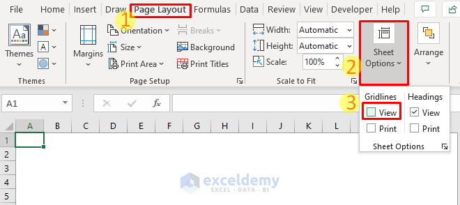
Click on Page Layout. Uncheck the View checkbox under Gridlines in the Sheet Options group. Excel will no longer display gridlines.
Things to Remember
When working with gridlines, keep these things in mind
- It is also possible to use the keyboard shortcut ALT + WVG (hold ALT and enter W V G). If the gridlines are visible, it will remove them, otherwise, it will make them visible.
- When the gridlines are removed from the worksheet, they will be removed from the entire worksheet. Each worksheet has its own setting. Despite removing the gridlines from one worksheet, they would still appear on all the others.
- Alternatively, you can remove the gridlines by filling the cells in the worksheet with a background color. The gridlines become invisible when you apply a fill color in a specific area, and you’ll notice that the fill color replaces the gridlines.
- Hold the Control Key and select the tabs to group all worksheets together, so you can remove the gridlines at once. There is a Group Mode active in the workbook (see the top of the workbook). All worksheets will now display gridlines, as soon as you change the gridlines view setting.
- It is not possible to print gridlines by default.
Download Practice Workbook
You can download the following practice workbook that we have used to prepare this article
Conclusion
In this tutorial, I have discussed 4 effective ways to change gridlines in Excel. I hope you found this article helpful. You can visit our website ExcelDemy to learn more Excel-related content. Please, drop comments, suggestions, or queries if you have any in the comment section below.
Get FREE Advanced Excel Exercises with Solutions!
