What Is the Time Value of Money?
The money that you have today is worth more than money you will receive in the future.
Parameters to Calculate Time Value of Money
- pv → pv the Present Value or the amount of money you currently have.
- fv → fv the Future Value of the money that you currently have.
- nper → nper represents the Number of Periods: Annually, Semi-Annually, Quarterly, Monthly, Weekly, Daily etc.
- rate → rate is the Interest Rate Per Year.
- pmt → pmt indicates Periodic Payments.
Note: In the Excel formula, the signs of PV and FV are opposite. PV is negative and FV is positive.
Example 1 – Using the FV Function to Calculate the Future Value of Money in Excel
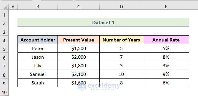
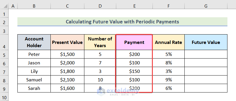
In the following dataset, initial investments (Present Value), the Annual Rate, and the Number of Years are displayed.
1.1 Future Value Without a Periodic Payment
Steps:
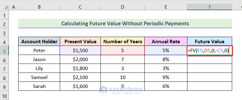
- Enter the following formula in F5.
=FV(E5,D5,0,-C5,0)Here,
E5 → rate
D5 → nper
0 → pmt
-C5 → pv
0 → 0 means payment is timed at the end of the period.
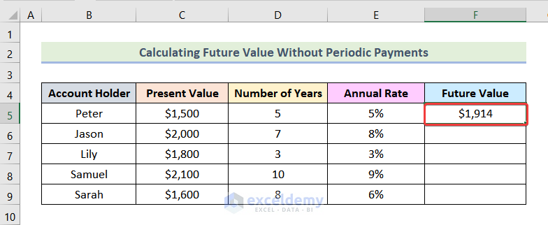
- Press ENTER.
This is the output.
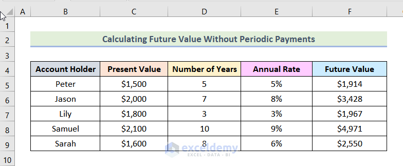
- Drag down the Fill Handle to see the result in the rest of the cells.
Read More: How to Calculate Periodic Interest Rate in Excel
1.2 Future Value with Periodic Payments
Steps:
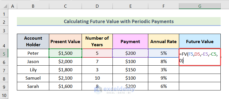
- Enter the following formula in G5.
=FV(F5,D5,-E5,-C5,0)Here,
F5 → rate
D5 → nper
-E5 → pmt
-C5 → pv
0 → 0 means payment is timed at the end of the period.
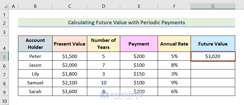
- Press ENTER.
This is the output.
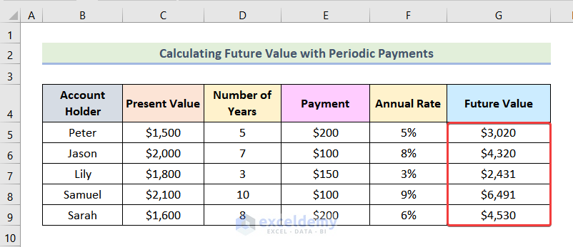
- Drag down the Fill Handle to see the result in the rest of the cells.
Read More: How to Apply Future Value of an Annuity Formula in Excel
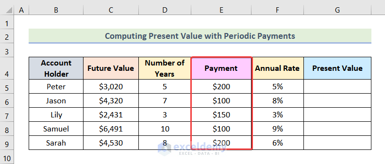
Example 2 – Computing the Present Value of Money with the PV Function
In the following dataset, Future Value, Annual Rate, and Number of Years are displayed.
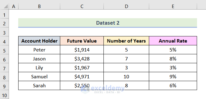
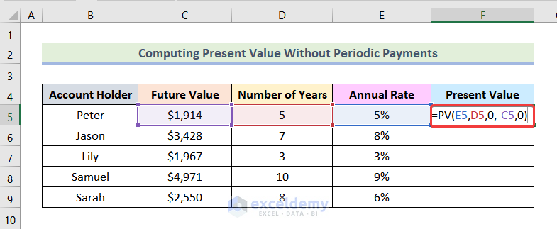
2.1 Present Value Without Periodic Payments
Steps:
- Enter the formula below in F5.
=PV(E5,D5,0,-C5,0)Here,
E5 → rate
D5 → nper
0 → pmt
-C5 → fv
0 → 0 means payment is timed at the end of the period.
- Press ENTER.
This is the output.
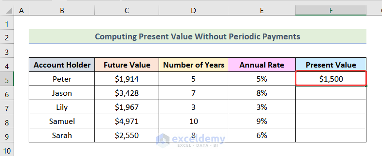
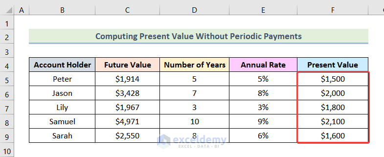
- Drag down the Fill Handle to see the result in the rest of the cells.
2.2 Present Value with Periodic Payments
Steps:
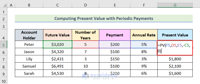
- Use the following formula in G5.
=PV(F5,D5,E5,-C5,0)Here,
F5 → rate
D5 → nper
E5 → pmt
-C5 → fv
0 → 0 means payment is timed at the end of the period.
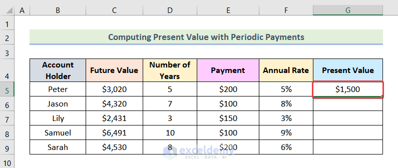
- Press ENTER.
This is the output.
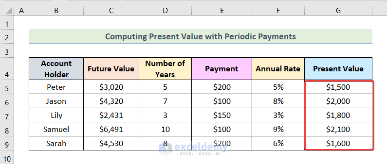
- Drag down the Fill Handle to see the result in the rest of the cells.
Read More: How to Apply Present Value of Annuity Formula in Excel
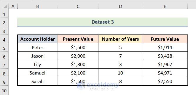
Example 3 – Calculating the Interest Rate with the RATE Function in Excel
In the dataset given below, Present Value, Future Value, and Number of Years are displayed.
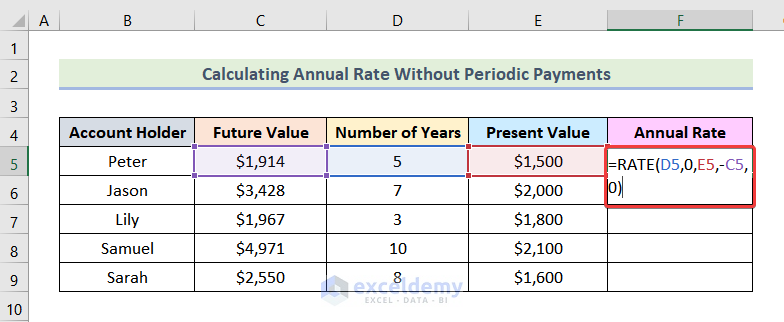
3.1 Interest Rate Without Periodic Payments
Steps:
- Enter the following formula in F5.
=RATE(D5,0,E5,-C5,0)Here,
D5 → nper
0 → pmt
E5 → pv
-C5 → fv
0 → 0 means payment is timed at the end of the period.
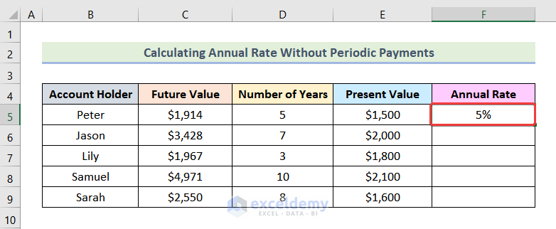
- Press ENTER.
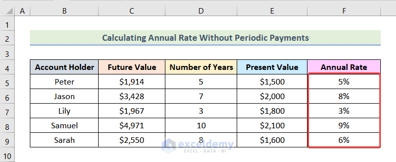
This is the output.
- Drag down the Fill Handle to see the result in the rest of the cells.
3.2 Interest Rate with Periodic Payments
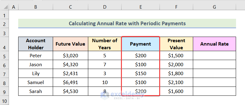
Steps:
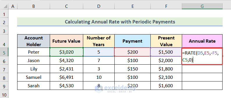
- Use the formula below in G5.
=RATE(D5,-E5,-F5,C5,0)Here,
D5 → nper
-E5 → pmt
-F5 → pv
C5 → fv
0 → 0 means payment is timed at the end of the period.
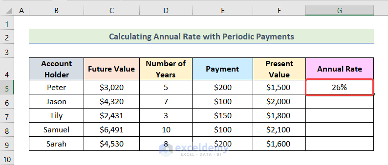
- Press ENTER.
This is the output.
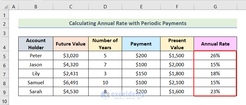
- Drag down the Fill Handle to see the result in the rest of the cells.
Read More: How to Calculate Present Value of Future Cash Flows in Excel
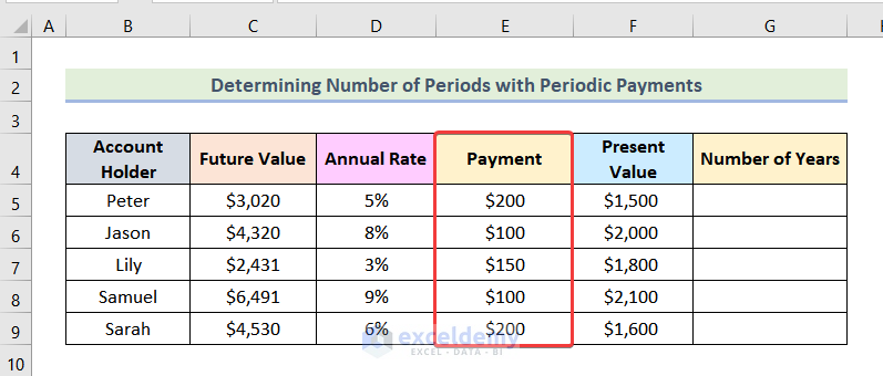
Example 4 – Computing the Number of Periods with the NPER Function
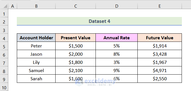
The following dataset showcases Present Value, Future Value, and Annual Rate.
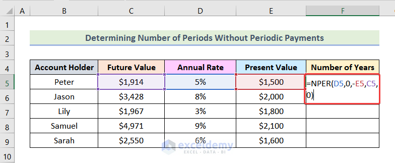
4.1 Number of Periods Without Periodic Payments
Steps:
- Enter the following formula in F5.
=NPER(D5,0,-E5,C5,0)Here,
D5 → rate
0 → pmt
-E5 → pv
C5 → fv
0 → 0 means payment is timed at the end of the period.
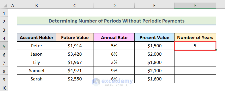
- Press ENTER.
This is the output.
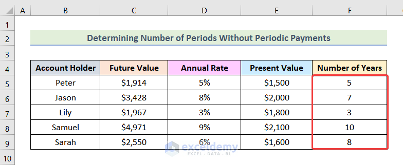
- Drag down the Fill Handle to see the result in the rest of the cells.
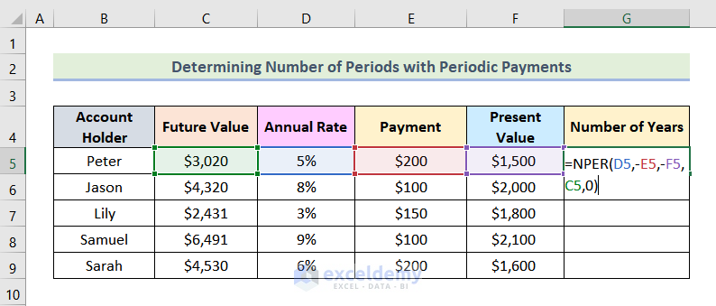
4.2 Number of Periods with Periodic Payments
Steps:
- Enter the following formula in G5.
=NPER(D5,-E5,-F5,C5,0)Here,
D5 → rate
-E5 → pmt
-F5 → pv
C5 → fv
0 → 0 means payment is timed at the end of the period.
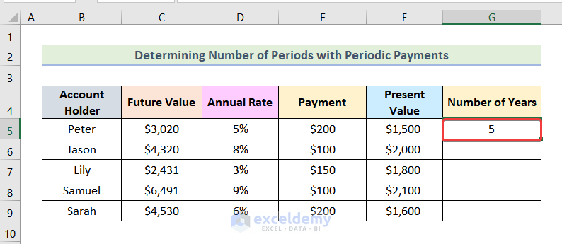
- Press ENTER.
This is the output.
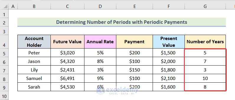
- Drag down the Fill Handle to see the result in the rest of the cells.
Read More: How to Calculate Present Value in Excel with Different Payments
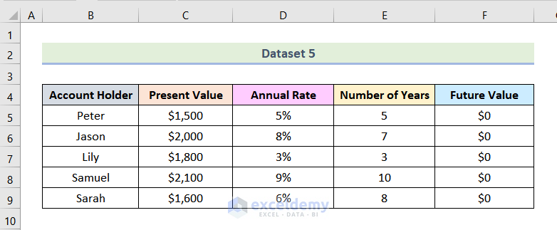
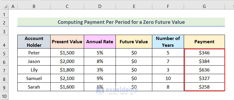
Example 5 – Using the PMT Function to Determine a Payment Per Period
In the dataset below, Present Value, Annual Rate, Number of Years, and Future Value are displayed.
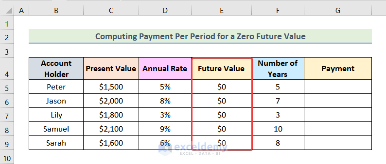
5.1 Payment Per Period for a Zero Future Value
Steps:
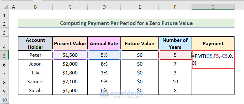
- Enter the formula below in G5.
=PMT(D5,F5,-C5,0,0)Here,
D5 → rate
F5 → nper
-C5 → pv
0 → fv
0 → 0 means payment is timed at the end of the period.
- Press ENTER.
This is the output.
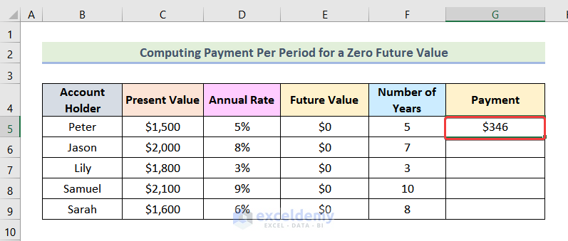
- Drag down the Fill Handle to see the result in the rest of the cells.
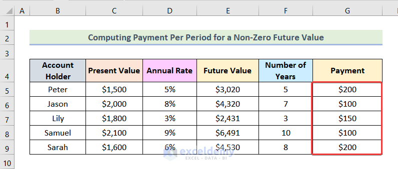
5.2 Payment Per Period for a Non-Zero Future Value
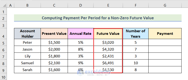
Steps:
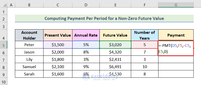
- Enter the following formula in G5.
=-PMT(D5,F5,-C5,E5,0)Here,
D5 → rate
F5 → nper
-C5 → pv
E5 → fv
0 → 0 means payment is timed at the end of the period.
- Press ENTER.
Note: The negative sign is used before the function, not to be displayed in the output.
This is the output.
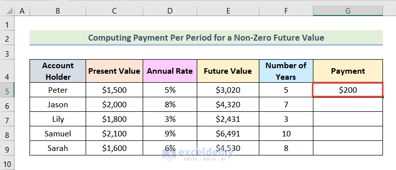
- Drag down the Fill Handle to see the result in the rest of the cells.
Read More: How to Calculate Future Value in Excel with Different Payments
How to Create a Time Value Money Table in Excel
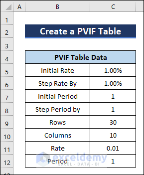
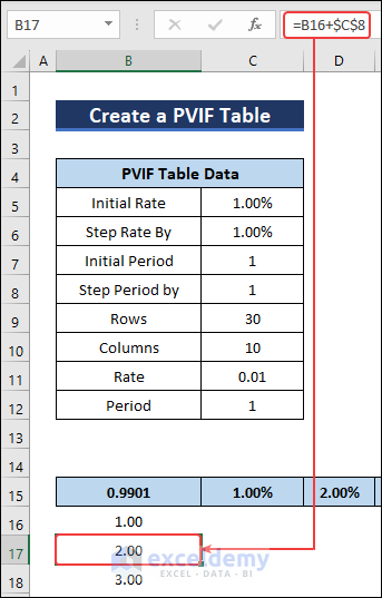
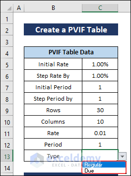
1. Create a PVIF Table
- Enter your data in the PVIF table.
- Go to B15 and enter the following formula.
=PV(C11,C12,0,-1)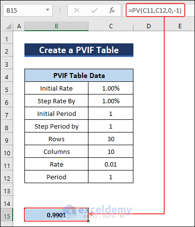
- Enter the Initial Rate in C15.
- Select D5 and enter the following formula to create the third column in the table. Drag the Fill Handle to column 16.
=C15+$C$6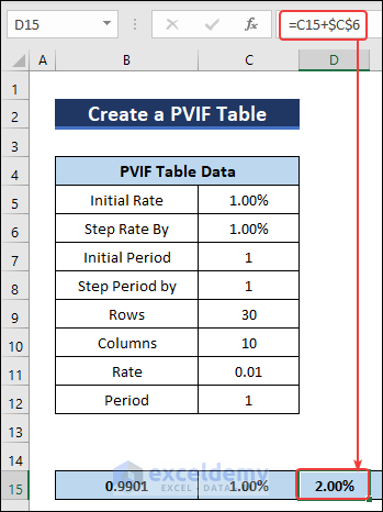
- Enter the Initial Period in B16.
- Add a new row by using the following formula in B17.
=B16+$C$8- Drag down the Fill Handle to see the result in the rest of the cells.
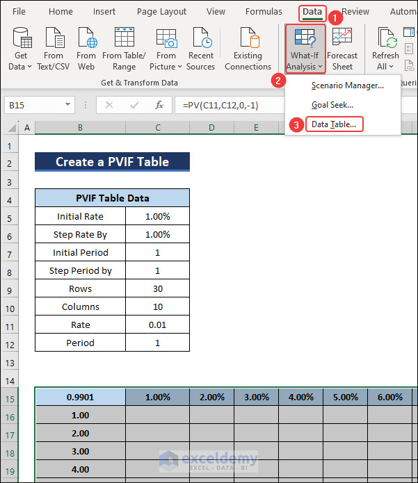
- Select the whole table (B15:L45).
- Go to Data >> What-If Analysis >> Data Table.
- In the Data Table, enter $C$11 as the Row input cell and $C$12 as the Column input cell.
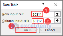
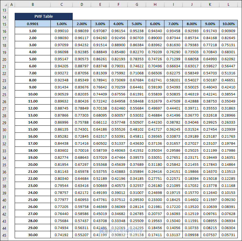
- Click OK and the PVIF table will be created.
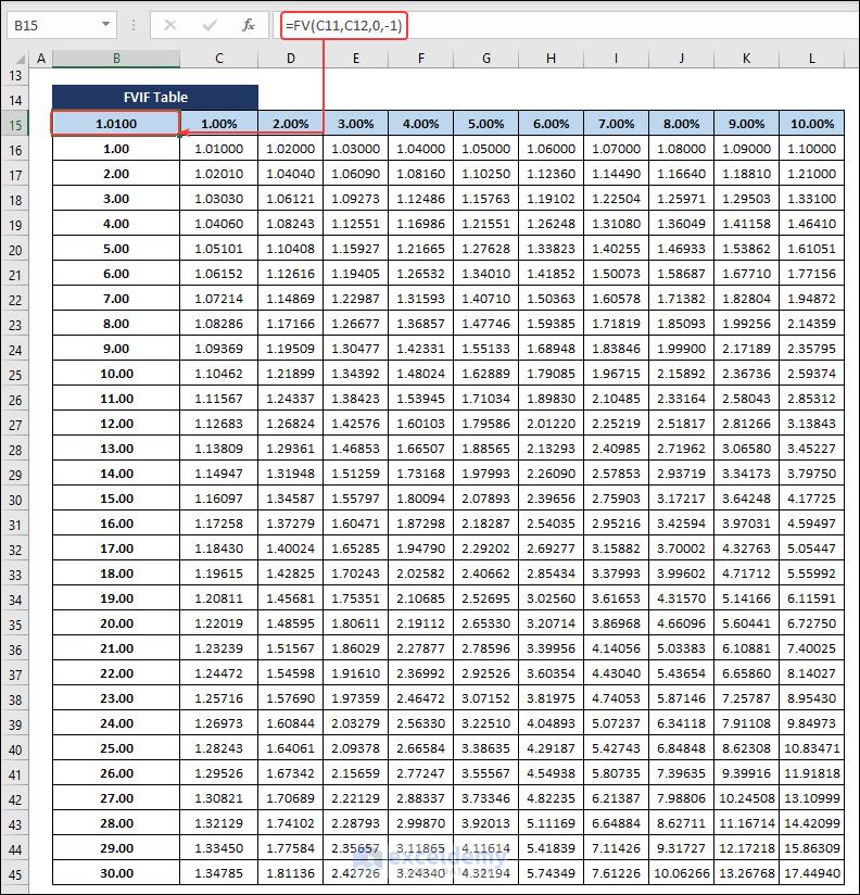
2. Make an FVIF Table to Calculate the Time Value of Money in Excel
The FVIF table contains future value interest factors.
- Copy the PVIF worksheet to a new worksheet.
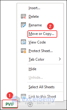
- Select B15 and enter the formula below.
=FV(C11,C12,0,-1)- Press Enter and you will have your FVIF table.
3. Calculating the Time Value of Money with a PVIFA Table
To calculate the present worth of future value as annuities.
- Add a new row: Type to the PVIFA table.
- Select C13 and go to Data >> Data Validation >> Data Validation.
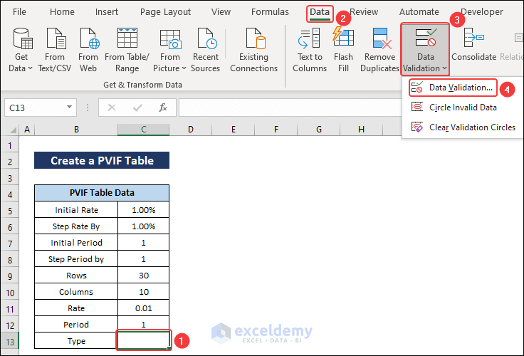
- Select List in Allow.
- Then enter “Regular, Due” in Source.
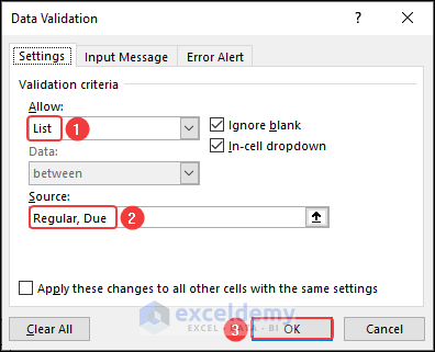
Two options will be added in C13.
- Enter the following formula in B16 and the PVIFA table will be created.
=IF(C13="Due",PV(C11,C12,-1,0,1),PV(C11,C12,-1,0,0))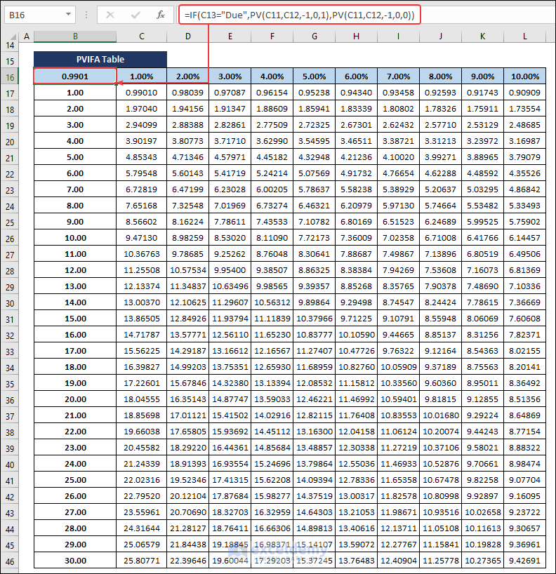
4. Create an FVIFA Table to Calculate the Time Value of Money in Excel
To determine the future worth of the present value of money.
- Copy the PVIFA table into a new sheet and change the formula of B16 to:
=IF(C13="Due",FV(C11,C12,-1,0,1),FV(C11,C12,-1,0,0))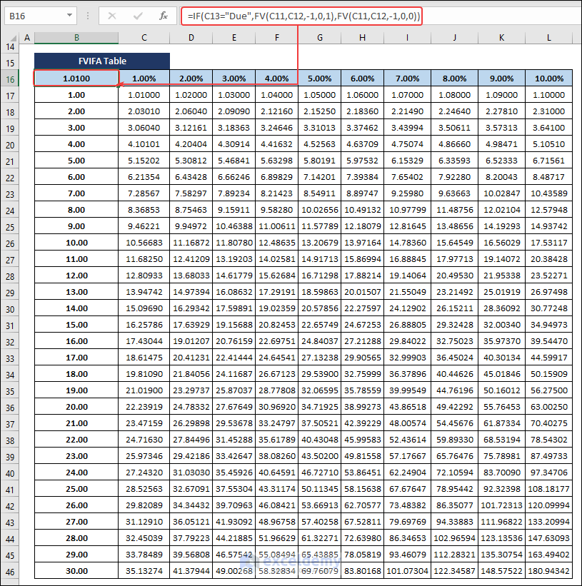
Download Practice Workbook
Related Articles
- How to Calculate Future Value of Growing Annuity in Excel
- Calculate Present Value of Lump Sum in Excel
- How to Calculate Present Value of Uneven Cash Flows in Excel
- Calculate Future Value of Uneven Cash Flows in Excel
Calculate Time Value of Money : Knowledge Hub
- Calculate NPV for Monthly Cash Flows with Formula in Excel
- How to Calculate Present Value of Future Cash Flows in Excel
- How to Calculate Future Value with Inflation in Excel
<< Go Back to Excel for Finance | Learn Excel
Get FREE Advanced Excel Exercises with Solutions!
