For illustration, we will use the sample dataset below.

Method 1 – Calculate Time Difference in Excel Using Operator
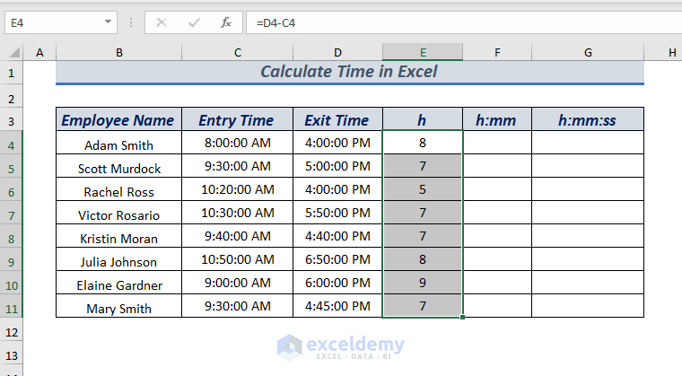
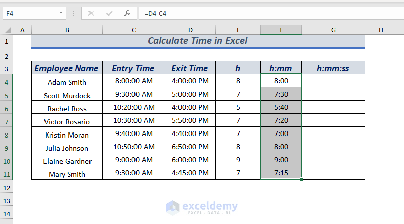
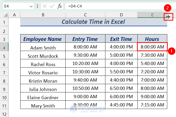
⏩ In cell E4, type the following formula.
=D4-C4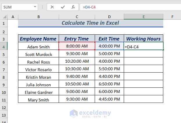
We selected D4 and C4 cells and then subtracted the C4 cell time from D4.
Press ENTER to get the time difference.
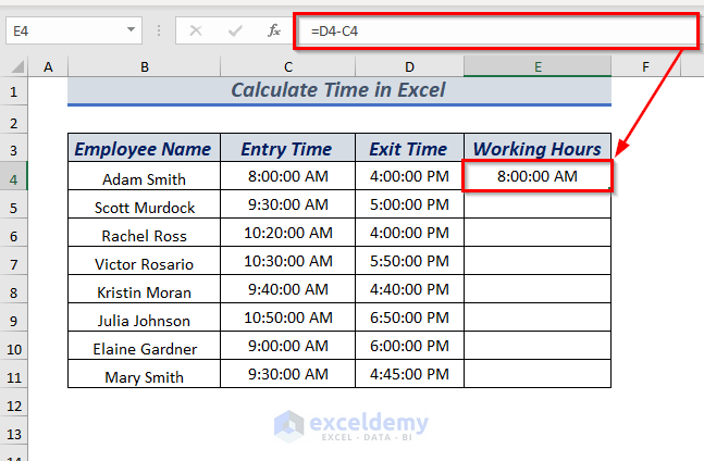
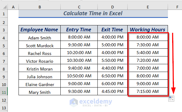
AutoFill the formula for the rest of the cells.
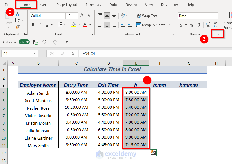
1.1. Change Time Format in h, h:mm and h:mm:ss format
Whenever we use an operator to get the time difference, the output is in the existing format. You have to change the format if you want it in a different format.
Select the cell or cell range that you want to change the format.
➤ I selected the cell range E4:E11.
Open the Home tab >> from Number group >> select the Number Format icon.
A dialog box will appear.
⏩ Select custom and type h.
Click OK.
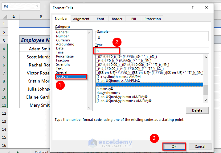
The selected cell range time will be converted to hours.
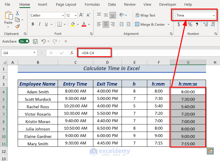
Select the cell or cell range that you want to change the format.
➤ I selected the cell range F4:F11.
Oopen the Home tab >> from Number group >> select the Number Format icon.
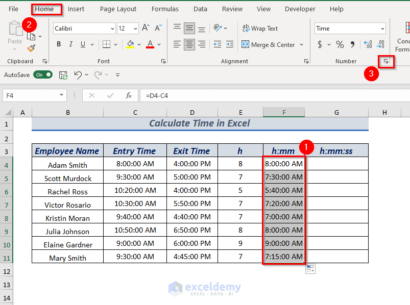
A dialog box will appear.
⏩ Select custom and type h:mm.
Click OK.
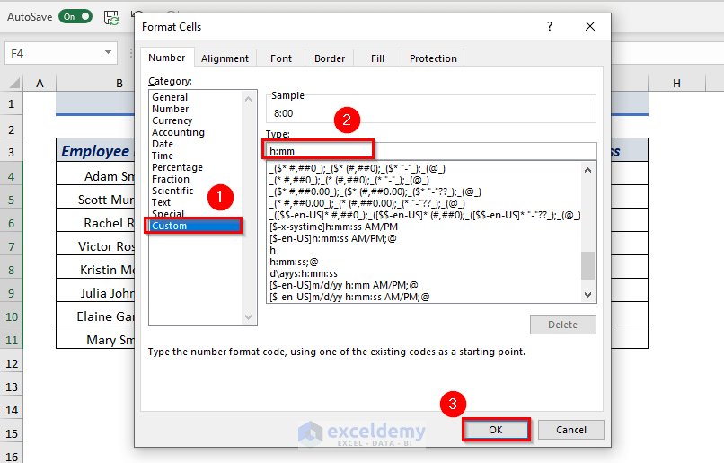
The selected cell range time will be converted into only hours & minutes.
Use the same process to convert the time into an hour, minute & second format.
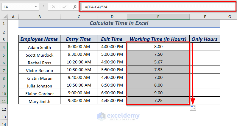
Method 2 – Calculate Time Difference in Hours
⏩ In cell E4, type the following formula.
=(D4-C4)*24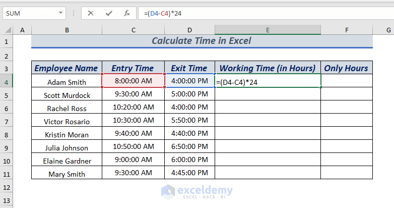
Press ENTER to get the time difference in hours.
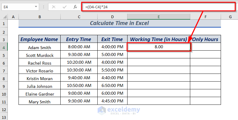
AutoFill the formula for the rest of the cells.
To get the hour without decimal values, use the INT function.
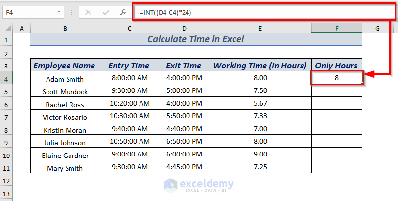
⏩ In cell F4, type the following formula.
=INT((D4-C4)*24)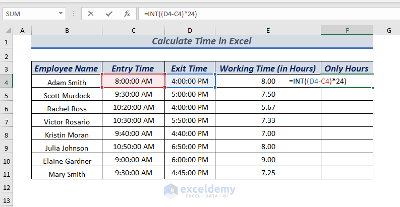
The INT function will return only the integer values.
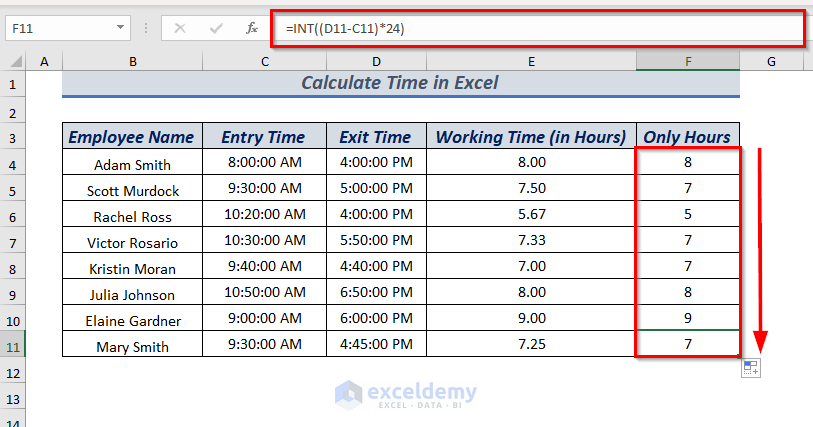
Press ENTER to get the time difference in integer hours.
AutoFill the formula for the rest of the cells.
To calculate the time difference in minutes, use this formula:
=(D4-C4)*24*60To calculate the time difference in seconds, use this formula:
=(D4-C4)*24*60*60Method 3 – Using Excel TEXT Function to Calculate Time Difference in Hours
⏩ In cell E4, type the following formula.
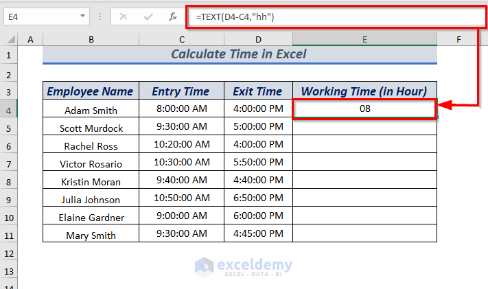
=TEXT(D4-C4,"hh")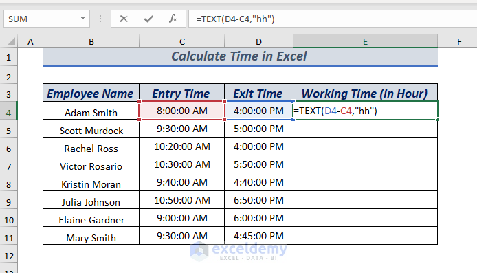
Press ENTER to get the time difference in hours.
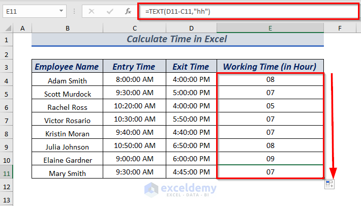
AutoFill the formula for the rest of the cells.
For more ways to calculate the time difference you can check the article How to Calculate Time Difference.
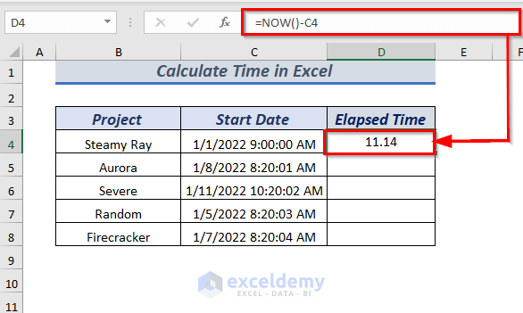
Method 4 – Calculating Elapsed Time Using Excel NOW Function
⏩ In cell D4, enter the following formula.
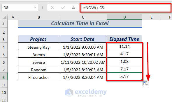
=NOW()-C4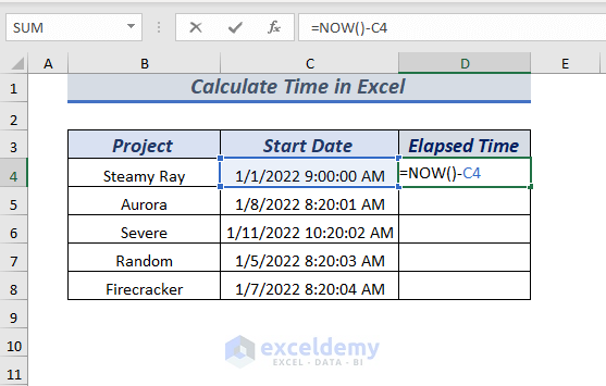
Press ENTER to get the elapsed time from the selected date.
AutoFill the formula for the rest of the cells.
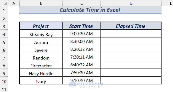
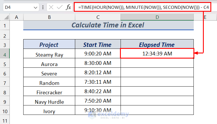
Method 5 – Calculating Elapsed Time Using TIME Function
In case your dataset contains only time values without dates, you will need to use the TIME function to calculate the elapsed time correctly.
⏩ In cell D4, type the following formula.
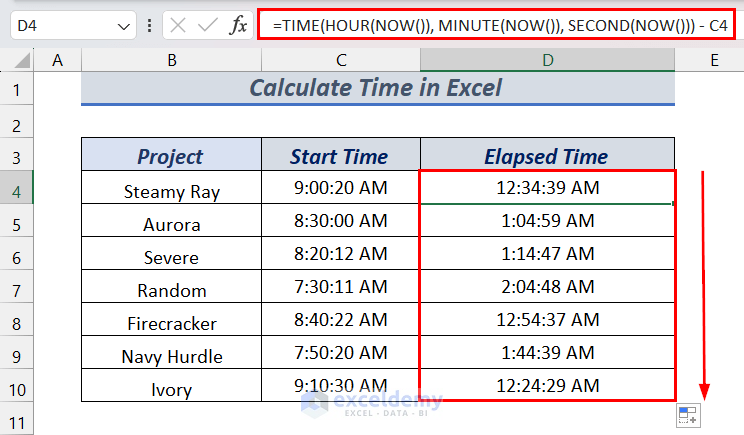
=TIME(HOUR(NOW()), MINUTE(NOW()), SECOND(NOW())) - C4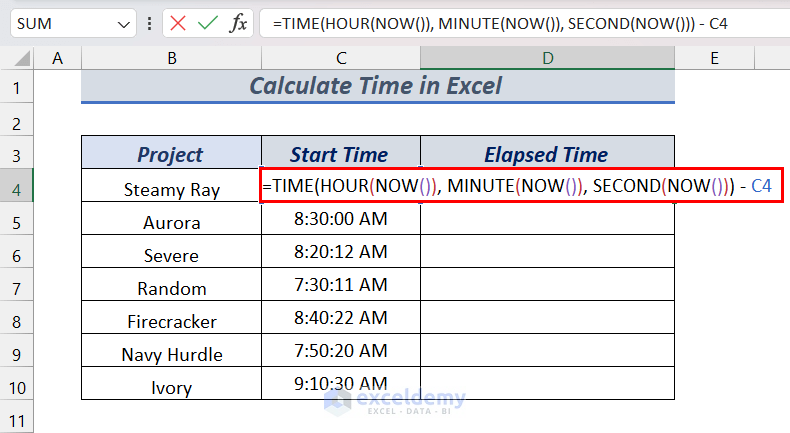
Press ENTER to get the elapsed time.
AutoFill the formula for the rest of the cells.
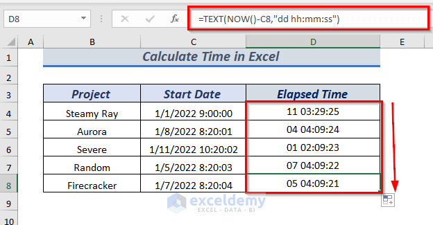
Method 6 – Calculating Elapsed Time Using Excel TEXT & NOW Function
⏩ In cell D4, type the following formula.
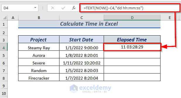
=TEXT(NOW()-C4,"dd hh:mm:ss")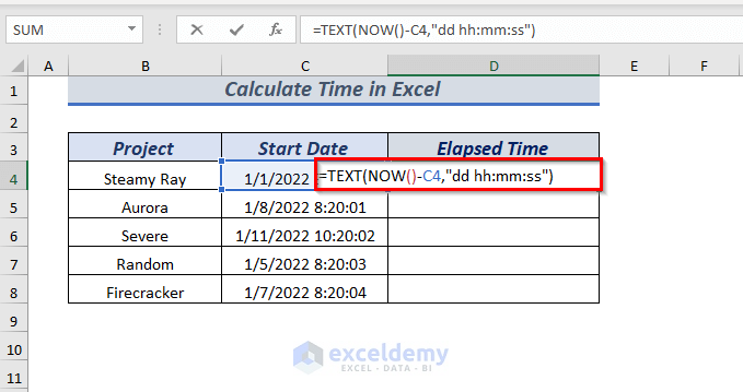
Press ENTER to get the time elapsed in days, hours, minutes, and seconds format.
AutoFill the formula for the rest of the cells.
Method 7 – Calculate & Show Time Difference
⏩ In cell D4, type the following formula.
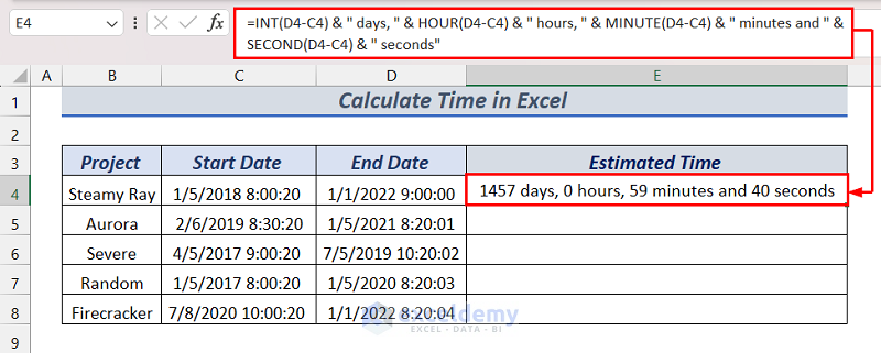
=INT(D4-C4) & " days, " & HOUR(D4-C4) & " hours, " & MINUTE(D4-C4) & " minutes and " & SECOND(D4-C4) & " seconds"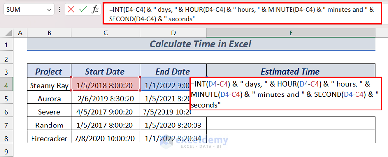
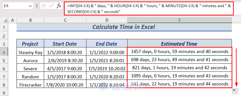
Press ENTER to get the time displayed in days, hours, minutes, and seconds text.
AutoFill the formula for the rest of the cells.
Method 8 – Dealing Negative Time
There is a possibility of getting ###### errors in Excel while dealing with negative times.
But there are ways to show negative times properly in Excel without getting this error.
8.1. Using IF Function to Calculate Negative Time
⏩ In cell E4, type the following formula.
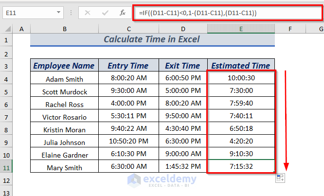
=IF((D4-C4)<0,1-(D4-C4),(D4-C4))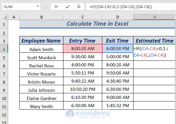
Here, in the IF function, I used (D4-C4)<0 as logical_test, 1-(D4-C4) as value_if_true, and (D4-C4) as value_if_false.
Now, if the logical_test value becomes TRUE then the IF function will return the time difference subtracted by 1 otherwise the positive time difference will remain as it is.
Press ENTER to get a positive time.
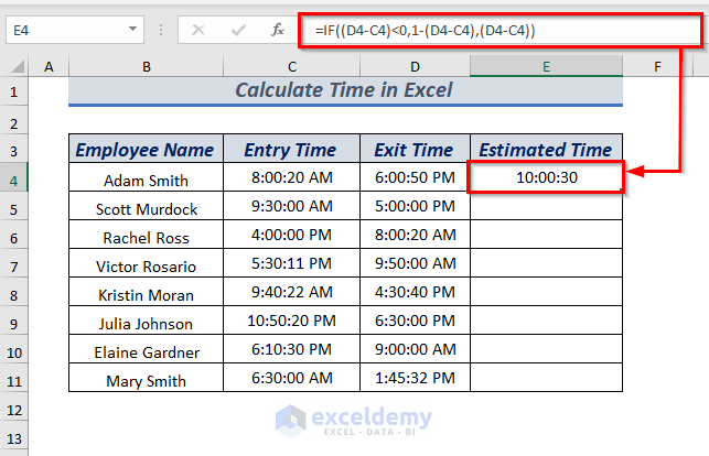
AutoFill the formula for the rest of the cells.
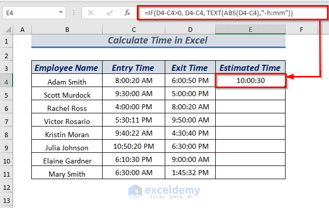
8.2. Using IF, TEXT & ABS Function to Calculate Negative Time
⏩ In cell E4, type the following formula.
=IF(D4-C4>0, D4-C4, TEXT(ABS(D4-C4),"-h:mm"))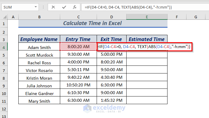
Press ENTER to get the negative time difference.
AutoFill the formula for the rest of the cells.
Method 9 – Adding Hours in Excel with TIME function
9.1. Add Time Under 24 Hours in Excel
⏩ In cell D4, type the following formula.
=C4 + TIME(8, 0, 0)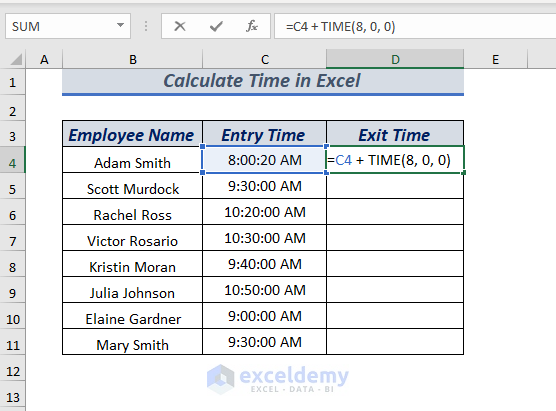
Here, in the TIME function, I used 8 as an hour and used 0 as a minute & second as I wanted to add only hours. Then added it with the time of cell C4.
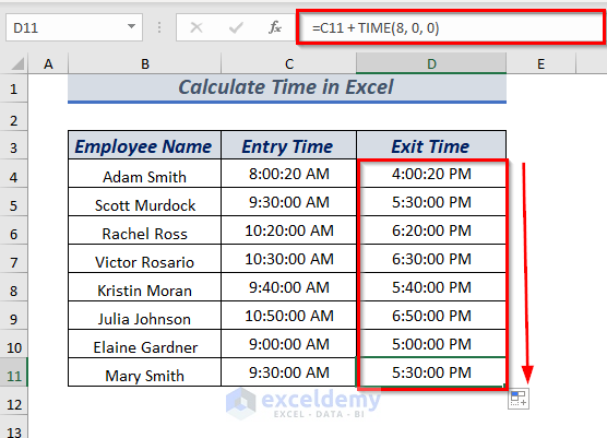
Press ENTER to get the added time.
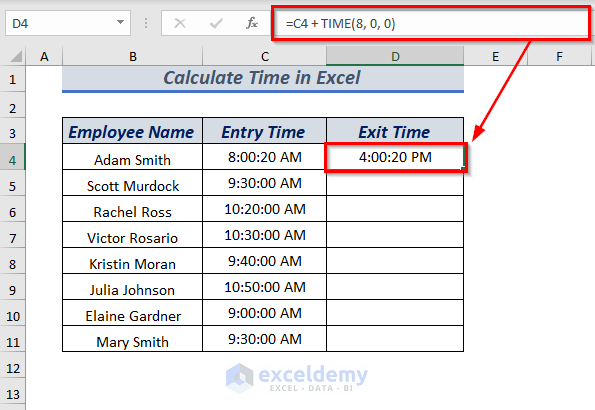
AutoFill the formula for the rest of the cells.
9.2. Add Time Under or Over 24 Hours in Excel
⏩ In cell D4, type the following formula and press enter.
=C4+ (48/24)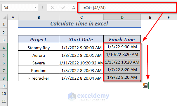
AutoFill the formula for the rest of the cells.
Method 10 – Adding Minutes in Excel
10.1. Add Time Under 60 Minutes in Excel
⏩ In cell E4, type the following formula.
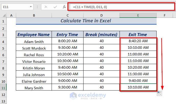
=C4 + TIME(0, D4, 0)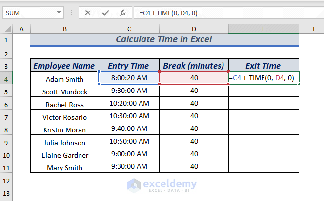
Press ENTER, and you will get added time.
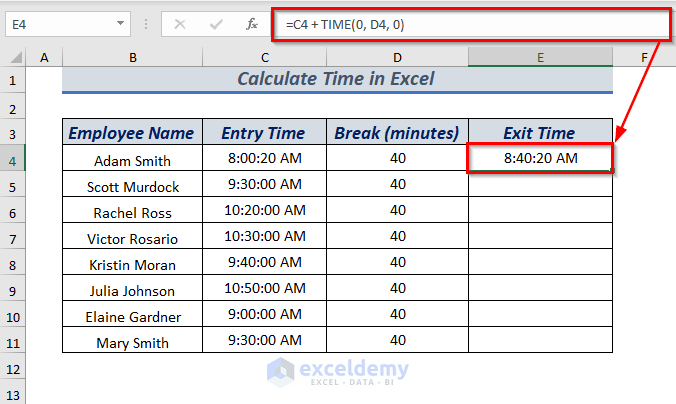
AutoFill the formula for the rest of the cells.
10.2. Add Time Under or Over 60 Minutes in Excel
⏩ In cell D4, type the following formula.
=C4+ (480/1440)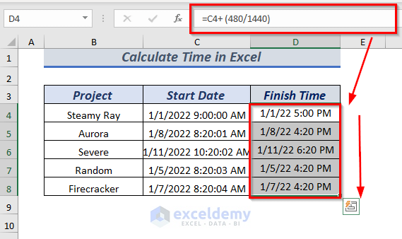
AutoFill the formula for the rest of the cells.
Method 11 – Adding Seconds in Excel
11.1. Add Time Under 60 Seconds
⏩ In cell E4, type the following formula.
=C4 + TIME(0, 0, D4)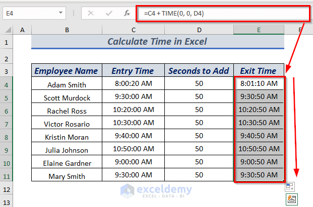
AutoFill the formula for the rest of the cells.
11.2. Add Time Under or Over 60 Seconds
⏩ In cell E4, type the following formula.
=C4+ (320/86400)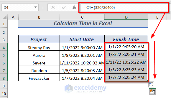
AutoFill the formula for the rest of the cells.
Method 12 – Subtract Hours in Excel
12.1. Subtract Time Under 24 Hours
⏩ In cell E4, type the following formula and press ENTER.
=C4 - TIME(D4, 0, 0)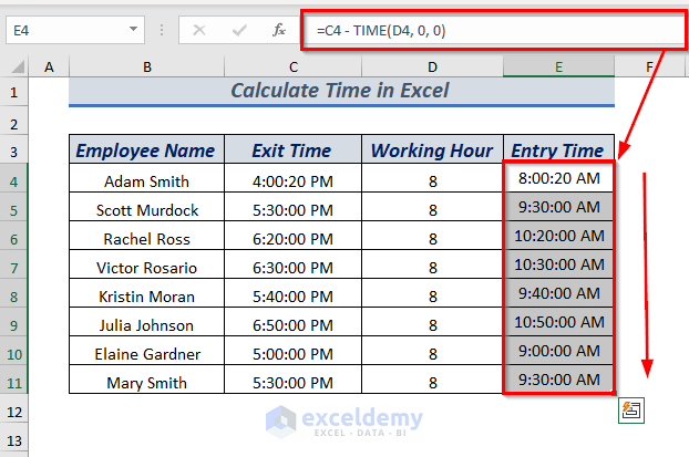
AutoFill the formula for the rest of the cells.
12.2. Subtract Time Under or Over 24 Hours
⏩ In cell D4, type the following formula.
=C4 - (48/24)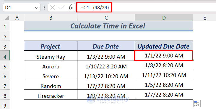
AutoFill the formula for the rest of the cells.
Read More: How to Subtract Time in Excel
Method 13 – Subtract Minutes in Excel
13.1. Subtract Time Under 60 Minutes
⏩ In cell E4, type the following formula and press ENTER.
=C4 - TIME(0, D4, 0)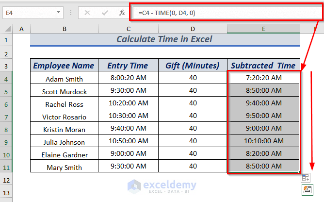
AutoFill the formula for the rest of the cells.
13.2. Subtract Time Under or Over 60 Minutes
⏩ In cell D4, type the following formula and press ENTER.
=C4- (480/1440)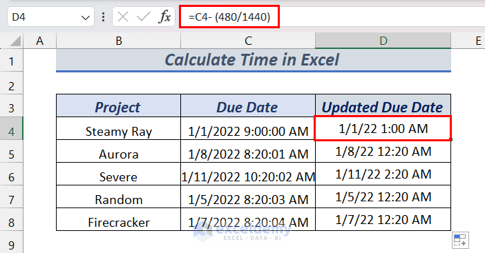
AutoFill the formula for the rest of the cells.
Method 14 – Subtract Seconds in Excel
14.1. Subtract Time Under 60 Seconds
⏩ In cell E4, type the following formula and press enter.
=C4 - TIME(0, 0, D4)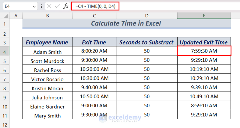
AutoFill the formula for the rest of the cells.
14.2. Subtract Time Under or Over 60 Seconds
⏩ In cell D4, type the following formula.
=C4 -(488/86400)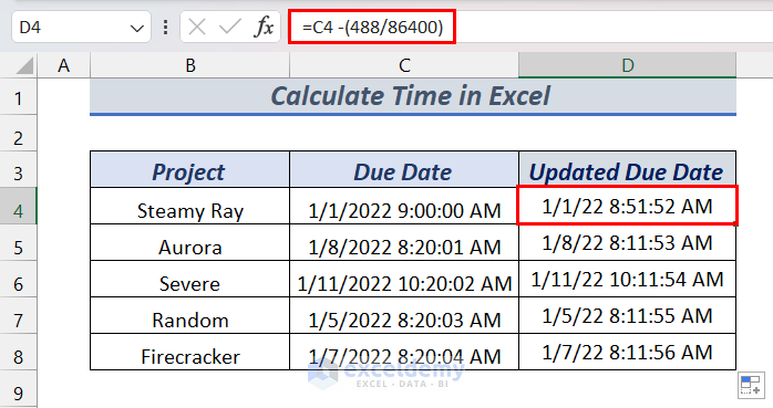
AutoFill the formula for the rest of the cells.
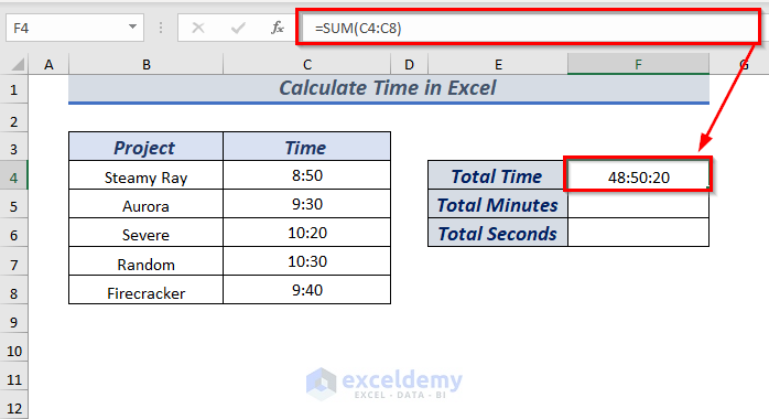
Method 15 – Calculate Total Time Using Excel SUM Function
⏩ In cell F4, type the following formula.
=SUM(C4:C8)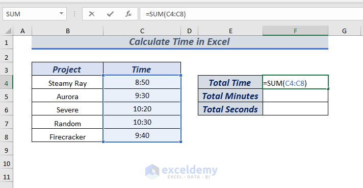
Press ENTER and you will get the total time.
15.1. Calculate Total Minutes Using SUM
Select the cell or cell range that you want to change the format.
➤ I selected cell F4.
Open the Home tab >> from Number group >> select the Number Format icon.
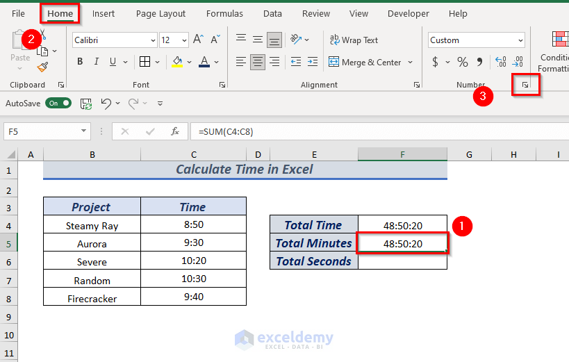
A dialog box will appear.
⏩ Select custom and type [mm] to get only minutes.
Click OK.
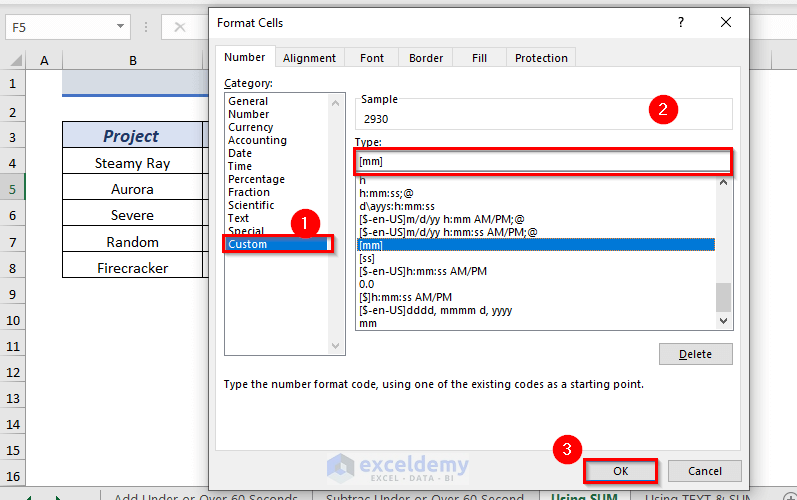
The selected cell time will be converted into minutes.
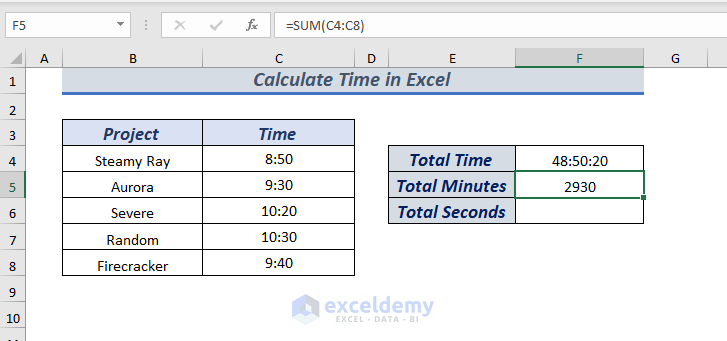
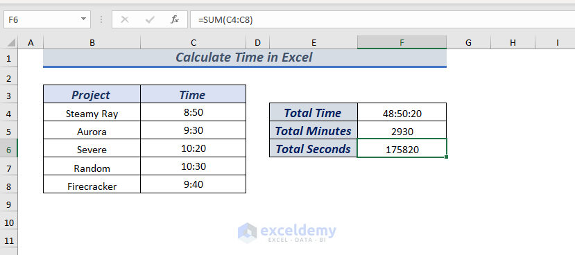
15.2. Calculate Total Seconds Using SUM
⏩ Select custom and type [ss] to only get seconds.
Click OK.
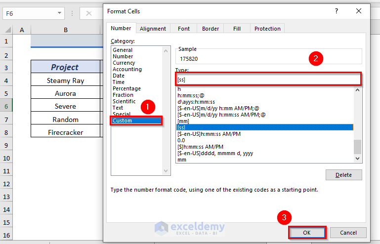
The selected cell time will be converted into seconds.
Method 16 – Using TEXT & SUM to Calculate Total Time
⏩ In cell F4, type the following formula.
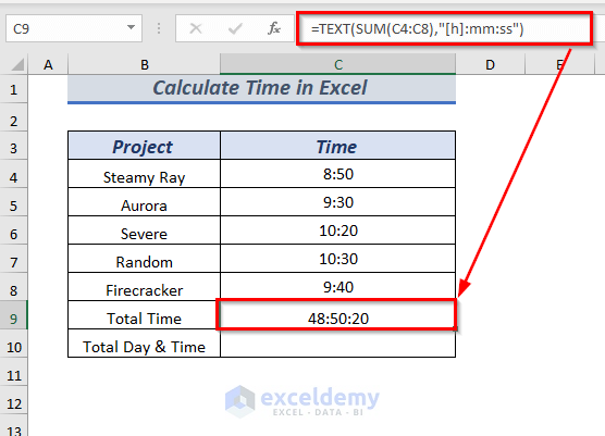
=TEXT(SUM(C4:C8),"[h]:mm:ss")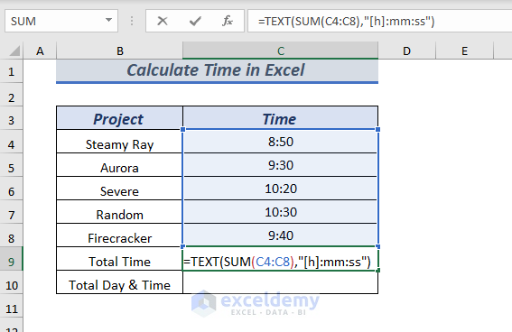
Press ENTER to get the formatted total time.
16.1. Using TEXT & SUM to Calculate Total Day & Time
⏩ In cell F4, type the following formula.
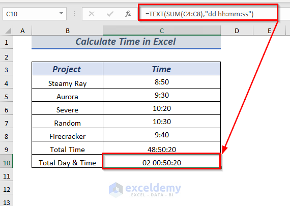
=TEXT(SUM(C4:C8),"dd hh:mm:ss")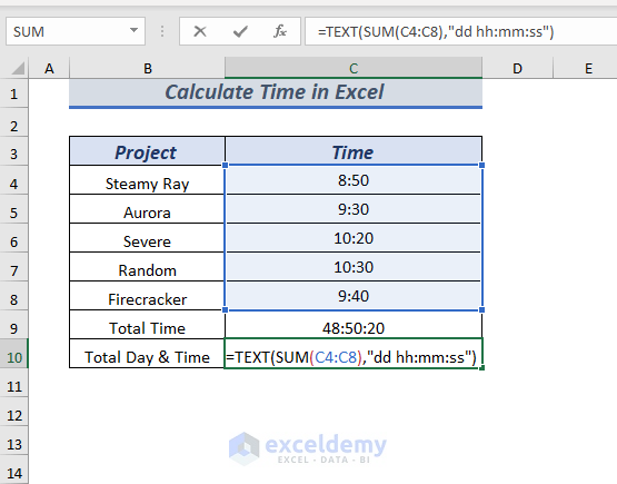
Press ENTER to get the formatted total time with the number of days.
Method 17 – How to Calculate Hours Worked in Excel
17.1 Using Simple Formula to Calculate Total Hours Worked
Insert the formula below in cell E4 >> press Enter key >> use the Fill Handle tool >> change the number format to the Number option.
=MOD(D4-C4,1)*24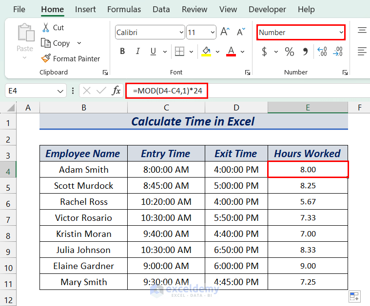
Here, we applied the MOD function to avoid returning negative numbers in case the end time is earlier then the start time.
17.2 Combining IF and SUM Functions to Calculate Overtime
In cell E4, insert the following formula >> press Enter key >> drag down the Fill Handle tool.
=IF((D4-C4)*24>$H$4,$H$4,(D4-C4)*24)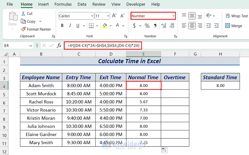
In cell F4, enter the following formula >> press Enter key >> drag down the Fill Handle icon. Don’t forget to change the number formatting to the Number option.
=IF((D4-C4)*24>$H$4,(D4-C4)*24-$H$4,0)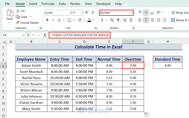
17.3 Calculate Hours Worked in a Weekly Timesheet
Insert the following formula in cell E4 >> press Enter key >> use the Fill Handle tool to copy the formula.
=(D4-C4)*24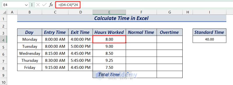
To calculate the overtime value for each workday, enter the following formula in cell G4 >> press Enter key >> drag down the Fill Handle icon.
=IF(SUM($E$4:E4)>$I$4,SUM($E$4:E4)-$I$4,0)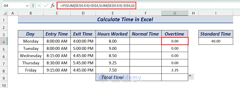
To calculate the normal time using the MAX function. Enter the following formula in cell F4 >> press the Enter key >> drag down the Fill Handle tool.
=MAX(E4-G4,0)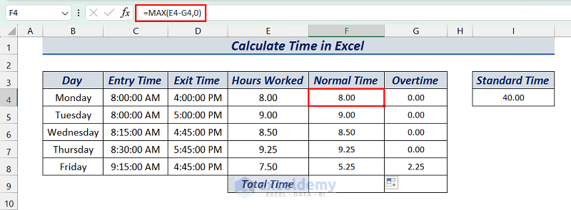
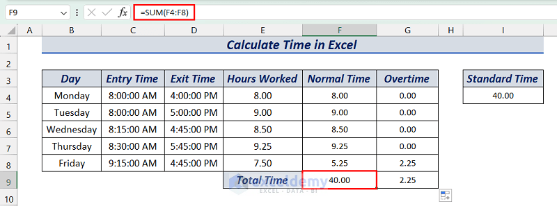
To find the total normal time and total overtime, insert the formula below in cell F9 >> press Enter key >> drag the Fill Handle tool to the right.
[Fixed] Results Showing Hash(#) Symbols Instead of Time or Date in Excel
In various instances of calculating time or date values, we get multiple Hash (#) symbols instead of the actual result. This can occur due to the column not being wide enough. In the following image, we have such a scenario.
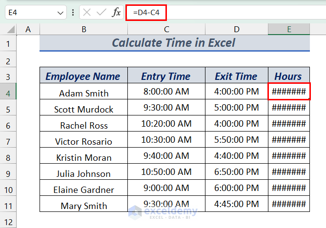
To fix this, adjust the column width and the actual outputs will be visible.
Download Practice Workbook
Calculate Time in Excel: Knowledge Hub
- Calculate On Time Delivery Performance
- How to Calculate Production per Hour
- Create an Injection Molding Cycle Time Calculator
- How to Get Average Time in Excel
<< Go Back to Date-Time in Excel | Learn Excel
Get FREE Advanced Excel Exercises with Solutions!
