How to Use Auto Filter and Advanced Filter in Excel

Today, we will discuss how to use Auto Filter and Advanced Filter in Excel. The Auto Filter is the default filtering option in Excel. It allows users to filter by any value and from any column. But it only allows users to filter with a maximum of 2 criteria. On the other hand, the Advanced Filter is user specific. Here, the users set the filtering criteria and one can see the criteria while filtering.

Auto Filter and Advanced Filter in Excel: 2 Distinct Methods

In this article, we will discuss the Auto Filter and Advanced Filter options in Excel. we will explain the usage of the Auto Filter command in the first method. In the second one, we will demonstrate the usage of the Advanced Filter option in different cases.

1. Using Auto Filter

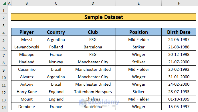
In the first method, we will show two ways of using the Auto Filter in Excel. Firstly, we will use the Filter command from the ribbon to do so. Then, we will use the FILTER function to get the job done. Here, we have a dataset that contains the information of 10 football players like, their County, the Club that they are playing in, their playing Position and their Birth Date. We will apply the Auto Filter and Advanced Filter feature on this dataset.

1.1 Using Filter Command

The Filter command is the default filtering tool in Excel. It allows user filter data quickly as well as with more versatility.

Steps:

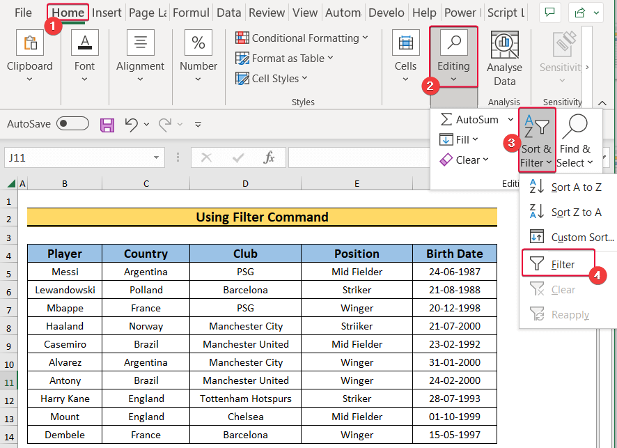
• Firstly, go to the Home
• Secondly, select Editing >> Sort & Filter >> Filter.
• As a result, a filter button will appear beside each column heading.

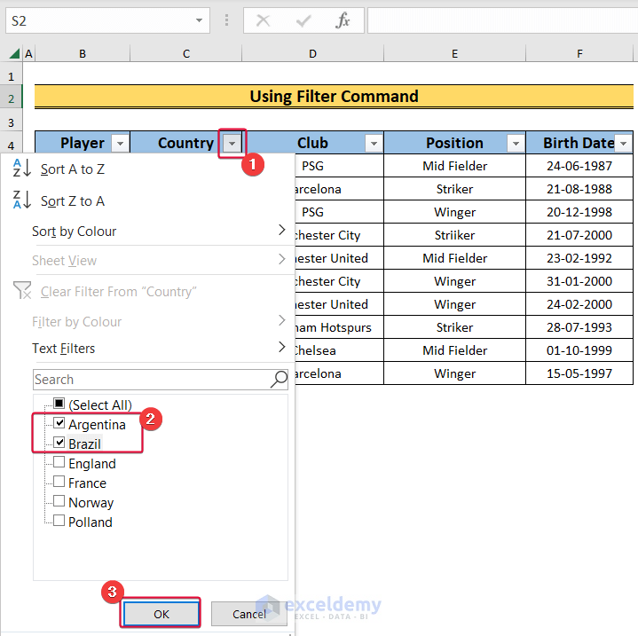
• Now, click on any of the filter buttons from any of the headings.
• Here, we will select the button beside the Country column.
• Next, we will filter the dataset by clicking on the data that we want to see from the dataset.
• Here, we will select Argentina and Brazil as our filter option.
• Finally, click OK.

• As a result, we will see the data of the players who are only from Brazil and Argentina.

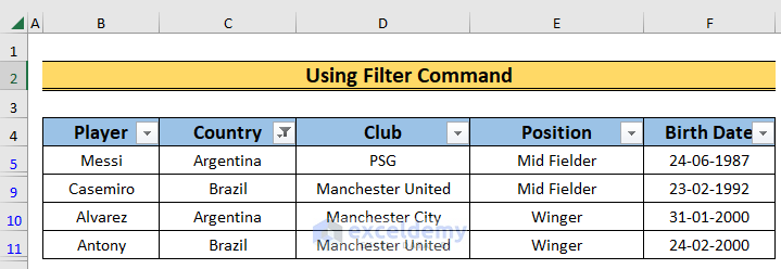
Thus, we will have our data filtered using the Filter command.

1.2 Applying FILTER Function

In this section, we will use the FILTER command to Auto Filter in Excel. The FILTER function takes the cell range through which it will filter and also the cell range where the criteria is present to filter the dataset.

Steps:

• First, click on the B16 cell and enter the following,

• Then, press Enter.
• As a result, Excel will return the data of only the Brazilian players.

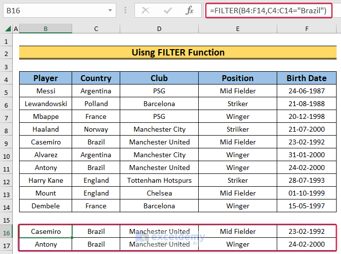
This is how we will use the Auto Filter feature in Excel.

2. Using Advanced Filter

In this following method, we will illustrate different usage of the Advanced Filter in Excel. We will use the feature on text values. We will then use AND and OR logics to filter data using the Advanced Filter option. Next, we will apply the Advanced Filter on a date range. Finally, we will show the use of the Advanced Filter with Wildcard.

2.1 Applying Advanced Filter on Text Values

In the first usage of the Advanced Filter, we will apply filtering on text values. We will look for exact and partial matches within the data and filter them accordingly.

2.1.1 Exact Match

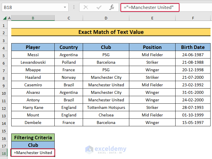
In this instance, we will filter the dataset based on text value with exact match from the dataset. So, the Advanced Filter will return only those values that will exactly match with our given text criteria.

Steps:

• To begin with, select the B18 cell and write,

• Then, press Enter.
• As a result, the exact match criteria will be set.

• Next, select Data >> Sort & Filter >> Advanced.
• As a result, the Advanced Filter prompt will be on the screen.

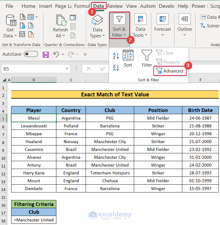
• In the prompt, first, choose Filter the list, in-place.
• Secondly, set the List range from B4 to F14.
• Thirdly, set B17:B18 as the Criteria range.
• Finally, click on OK.

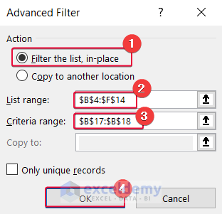
• As a result, Excel will return the data which contains exactly Manchester United.

This is how we will exactly match our criteria with our dataset in Advanced Filter.

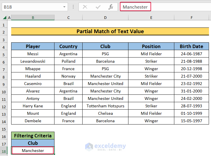
2.1.2 Partial Match

In this instance, we will partially match the text value in the criteria range with the values in the filter range. The Advanced Filter feature will return all the results that partially match with the criteria range.

Steps:

• To begin with, write “Manchester” in the B18 cell.
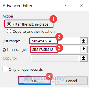
• Next, open the Advanced Filter prompt like the Exact Match method.

• In the prompt, first, mark the Filter the list, in-place oval.
• Secondly, choose B4:F14 as the List Range.
• Thirdly, select B17:B18 as the Criteria Range.
• Finally, hit OK.

• As a result, we will see all the results that include Manchester.

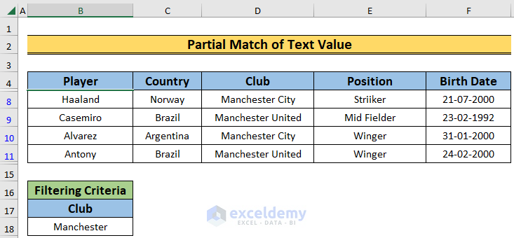
In the previous method, the Advanced Filter only returned the values that matched exactly with Manchester United. However, in this method, we get all the values that include Manchester.

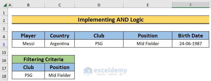
2.2 Implementing AND Logic in Advanced Filter

We can implement the AND logic in Advanced Filter if we keep all the filtering criteria in the same row. Here, we will place the Club and Position criteria side-by-side to implement the AND logic.

Steps:

• Firstly, choose the B18 cell and write PSG in it.

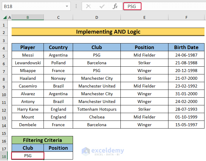
• After that, select the C18 cell and type Mid Fielder as the next criteria.
• Now, open the Advanced Filter prompt like the Previous Methods.

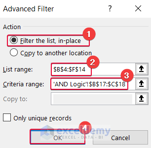
• In the prompt, first, select the Filter the list, in-place option.
• Then, choose B4:F14 as the List Range.
• Thereafter, select B17:C18 as the Criteria Range.
• Finally, press OK.

• As a result, we will get the data of the player who is a Mid Fielder and plays for PSG.

Here, the two criteria are in the same row which invokes the AND logic. So, we get our filtered data from AND logic.

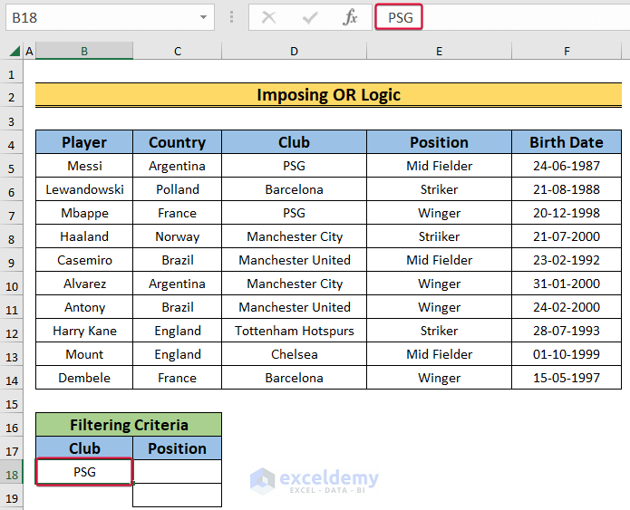
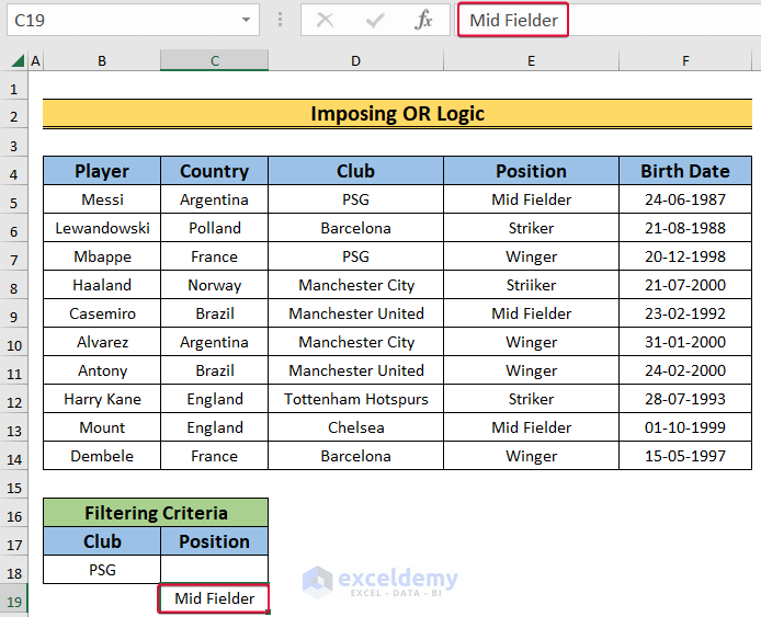
2.3 Imposing OR Logic in Advanced Filter

Here, we will impose the OR logic by typing the two criteria ranges in two different rows. We will write values of the criteria Club and Position in two different rows to get the OR logic.

Steps:

• At the start, write down PSG in the B17 cell.

• Next, write Mid Fielder in the B19 cell as the next criteria.
• Now, open the Advanced Filter prompt by following the steps from the Exact Match method.

• In the prompt, first, click on the Filter the list, in-place oval.
• Next, write B4:F14 in the List Range box.
• Then, select B17:C19 as the Criteria Range.
• Finally, hit OK.

• Consequently, we will get the data of the players who either plays for PSG or a Mid Fielder or both.

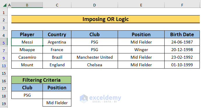
In this case, the Club and the Position criteria are in different rows which invokes the OR logic and so we get our filtered data by imposing the OR logic.

2.4 Using AND and OR Logic Together

In this section, we will merge the AND and OR logic together to filter our dataset. We will write two criteria in the same row to impose the AND logic and write another criterion in another row to apply the OR logic.

Steps:

• First, choose the B18 cell and write PSG as the first criteria.

• Next, select the B19 cell and type Mid Fielder to impose the OR logic.

• Finally, write Argentina in the D18 cell, same row as the first criterion, to implement the AND logic.
• After that, open the Advanced Filter prompt.

• Now, mark the Filter the list, in-place box.
• Next, choose B4:F14 as the List Range.
• After that, select B17:D19 as the Criteria Range.
• Finally, hit OK.

• As a result, we will get the players’ data who are either a PSG Mid Fielder or a Mid Fielder.

This is how we can use the AND and OR logic together.

2.5 Applying Advanced Filter on Date Range

We can also apply the Advanced Filter on dates. Here, we will filter out the players’ data who were born after 1 January,1998 by using the Advanced Filter.

Steps:

• At the start, choose the B18 cell and enter >1/1/1998.
• Next, open the Advanced Filter prompt like the previous methods.

• In the prompt, first, check the Filter the list, in-place box.
• Next, choose B4:F14 as the List Range.
• Afterward, select B17:B18 as the Criteria Range.
• Finally, click on OK.

• Consequently, we will get the players’ profiles who were born after 1 January,1998.

Here, >1/1/1998 means all the dates that come after that date. So, we get the information of the players who were born after that date.

2.6 Using Advanced Filter with Wildcard

In the final method, we will use the Wildcard in the Advanced Filter’s criteria range to partially match any text value.

Steps:

• At the beginning, choose the B18 cell and enter *M*.
• Next, open the Advanced Filter prompt.

• In the prompt, first, mark the Filter the list, in-place box.
• Secondly, choose B4:F14 as the List Range.
• Thirdly, select B17:B18 as the Criteria Range.
• Finally, hit OK.

• Consequently, we will get the players’ data from Manchester United, Manchester City, and Tottenham Hotspurs.

The *=M means that the Advanced Filter will look for any values within the Club column that has an M and the asterisk sign in both the side of the M means it will also look for any sequences before and after that. That is why it picked the two Manchester clubs. In case of Tottenham, it has found “Tottenha” before the “m” and “Hotspurs” after the “m” and returned the whole thing.

Download Practice Workbook

You can download the practice workbook here.

Conclusion

In this article, we have talked in detail about the Auto Filter and Advanced Filter in Excel. This article will allow users to filter their data more efficiently and effectively. If you have any questions regarding this essay, feel free to let us know in the comments.

<< Go Back to Advanced Filter | Filter in Excel | Learn Excel