Latest Posts From Soumik Dutta

To demonstrate, we have a dataset of 5 students. Their name, department, examination marks, grades, DOB, and retake examination marks are in the range of cells ...

Method 1 - Applying CONCATENATE Function Steps: Select cell C5. Write down the following formula in the cell. Make sure that you input the Absolute ...

Method 1 - Using Simple User-Defined Function Steps: Go to the Developer tab and click on Visual Basic. If you don’t have that, you must display the ...

Method 1 - Inserting an Image from Your Device Steps Select the desired cell (e.g., C5). Go to the Insert tab. Click the drop-down arrow under ...
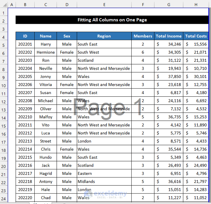
The sample dataset contains 21 employees in the range of cells B4:H25. Looking at Page Break Preview shows that the table is broken over two pages. ...
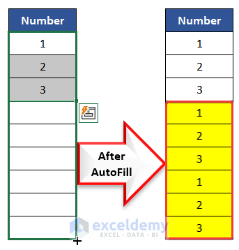
In this article, we will demonstrate four simple approaches to Autofill a series of sequential numbers repeatedly in Excel. The dataset below has 3 sequential ...

Method 1 - If Checkbox Is Checked, Set Cell Value Steps: Go to the Developer tab. If you don’t have it, enable the Developer tab on ribbon from Excel ...

In our everyday use of Microsoft Excel, it is important to visualize data. Sometimes it is enough to follow and measure the trend instead of going through ...

Example 1 - Creating Simple Gantt Chart with Conditional Formatting Steps: Enter the dates 1 July-15 July in the range of cells E4:S4. Select ...

The Excel Pie chart is a familiar figure to all of us. We use this type of chart to visualize the total amount in percentage. Like every type of chart, a pie ...

Excel charts are a familiar figure to all of us. Among them, the Bar chart is a pretty common one. In our regular life, we use it to show the data pattern ...

Legends are mainly used to denote the data series in an Excel chart for the convenience of our users. Sometimes, we need to show only values in the chart ...
Method 1 - Utilizing Excel Shapes Steps: Select the range of cells B5:C10. In the Insert tab, click on the drop-down arrow of the Insert Scatter (X, ...

Step 1: Design Primary Summary Layout Select cell B2 and enter the title of this sheet Summary. Rename the sheet name in the Sheet Name ...

In our regular professional life, we have to fill many series based on extrapolation to fulfill our organization's requirements. Using Microsoft Excel, we can ...
- « Previous Page
- 1
- …
- 3
- 4
- 5
- 6
- 7
- …
- 9
- Next Page »
See Our Reviews at


Hi Steven Leblanc
Thanks for your comment. In this article, all the operations are done using Microsoft Office 365 application. That’s why you got a different type of result after using the TEXTJOIN function. If you want to get a similar type of result just like us, you have to update your application from Excel 2019 to Office 365.
Hi Tom R,
Thanks for your comment. The numeric values are not a big issue. Our main focus is to demonstrate the procedure so that you can understand it and implement it in your regular life. Moreover, we also recommend our users download our Excel workbook first to overcome such misunderstandings.
However, we are providing an updated image of that part for your convenience.
Hi Martyn Kenyon,
Thanks for your suggestion regarding this issue. We hope that it will help others to resolve their problem.
If you have any further queries or suggestions feel free to share them that us through comments or email to our problem-solving team.
Hi, DIEGO.
Thank you for your concern. Yes, there is a way to exclude some tabs and merge only the tabs that you want. The generic code for this is:
Sub Merge_Multiple_Sheets()
Row_Or_Column = Int(InputBox(“Enter 1 to Merge the Sheets Row-wise.” + vbNewLine + vbNewLine + “OR” + vbNewLine + vbNewLine + “Enter 2 to Merge the Sheets Column-wise.”))
Merged_Sheets = InputBox(“Enter the Names of the Worksheets that You Want to Merge. Separate them by Commas.”)
Merged_Sheets = Split(Merged_Sheets, “,”)
Sheets.Add.Name = “Combined Sheet”
Dim Row_Index As Integer
Dim Column_Index As Integer
If Row_Or_Column = 1 Then
Column_Index = Worksheets(1).UsedRange.Cells(1, 1).Column
Row_Index = 0
For i = LBound(Merged_Sheets) To UBound(Merged_Sheets)
Set Rng = Worksheets(Merged_Sheets(i)).UsedRange
Rng.Copy
Worksheets(“Combined Sheet”).Cells(Row_Index + 1, Column_Index).PasteSpecial Paste:=xlPasteAllUsingSourceTheme
Row_Index = Row_Index + Rng.Rows.Count + 1 – 1
Next i
Application.CutCopyMode = False
ElseIf Row_Or_Column = 2 Then
Row_Index = Worksheets(1).UsedRange.Cells(1, 1).Row
Column_Index = 0
For i = LBound(Merged_Sheets) To UBound(Merged_Sheets)
Set Rng = Worksheets(Merged_Sheets(i)).UsedRange
Rng.Copy
Worksheets(“Combined Sheet”).Cells(Row_Index, Column_Index + 1).PasteSpecial Paste:=xlPasteAllUsingSourceTheme
Column_Index = Column_Index + Rng.Columns.Count + 1
Next i
Application.CutCopyMode = False
End If
End Sub
When you’ll run the code, it’ll ask for two inputs. Enter 1 if you want to merge the sheets row-wise, or 2 if you want to merge them column-wise.
And in the second input box, enter the name of the sheets that you want to merge. Don’t forget to put commas between the names, and don’t put any space after the commas.
Once you are done entering the inputs, click OK. You’ll find your selected tabs merged row-wise or column-wise in a new sheet called “Combined Sheet”.
Good luck.
Hi Mikekelly
Thanks for your query.
The ‘Ctrl+J’ command doesn’t replace the line break. It represents the line break feature when we use the Find & Replace dialog box to find this character. Now, If you look at our dataset, it was designed with multiple line breaks in a column. So, I hope that both datasets follow the same characteristic. To eliminate the line breaks from your sheet, you can go through the methods mentioned in this article. Among them, methods no 2, 3, and 4 are pretty simple and convenient. Moreover, in these methods, you do not have to deal with the ‘Ctrl+J’ command.
Let us know whether you can solve the issue. Please feel free to share with us if you have any further queries.
Hi Yenny,
Thanks for your query.
You can use the calculated items option only for those fields which are available in our pivot table. Because if the field did not show in the pivot table, the corresponding field will also not show in the item section of the dialog box, which appears after clicking on Fields, Items, & Set,
Thanks for your comment. We are very pleased to know that you find this article useful for you. As far as I know, Excel doesn’t have any built-in feature which can resolve your problem.
I recommend that you can set the first line of every MS Word page as a heading. This feature will help you see the text in the Navigation Panel of MS Word. As a result, you don’t need to scroll down all pages. You will just click on each text, then select the text and manually copy that into your Excel workbook.
Hi, Mark
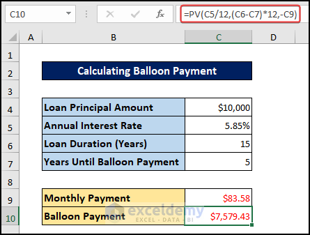
Thanks for your query. This might be a 1-60 months problem. Moreover, the complete scenario is a presumption of the author. So, the loan payment conditions may not be similar to the day-to-day practice situation. If you have specific terms and conditions in your loan statement, you can send that to our problem-solving team. They will help you to fulfill your requirement.
Hi Tim,
Thanks for your query. You are right. The combination of UNIQUE and RANDARRAY functions sometimes provide us with less than 10 number due to the duplicates. But, most of the time, it shows the 10 unique numbers on your first attempt. So, if you get less than 10 values, delete them and input the formula again. Once you get the 10 numbers, please copy and paste them in Value format asap to terminate further modification.
Moreover, you can also look to our other methods if your dataset provides you with such flexibility to use them.
Hi Amelie,
Thanks for your comment. As your dataset doesn’t follow any regular pattern, so I think we need an additional column to solve this issue. The procedure is:
1) First, insert a new column just right after your data column.
2) Then, at the first cell of that column, write down ‘[Value].
Here, the [Value] represents the data of the previous column.
3) Now, double-click on the Fill Handle icon.
4) The same result will be pasted on every cell. Click on the Auto Fill Options > Flash Fill option.
5) The apostrophe will add to every cell value, and it will prevent the disappearance of zero (0) from your dataset.
I hope you will be able to restore your cell values accurately. Please inform us if you are still facing any trouble.
Hi Brennan,
Thanks for your comment. You cannot use any function in the ‘criteria’ field of the COUNTIF function. You must have to input a specific text or value. Moreover, you have to mention a range of cells in the ‘criteria_range 1’ field, where the function count for your desired data. If you input a single cell instead of a range of cells, the COUNTIF function will not show the sum of the total count.
You can consider some other Excel functions like VLOOKUP and TODAY functions to get the decision if your worksheet allows you to place the value of cells L5, O5, R5, U5, X5, and AA5 in the conjugative cells whether row-wise or column-wise. I am telling you the process below.
First, set two criteria. As you want to show the value less or equal to 90 days, so you can set 90 for <= 90 days and 91 for >90 days.
Then, using the VLOOKUP and TODAY functions, write down the formula:
=VLOOKUP(TODAY()-[Cell Ref],Criteria,2,TRUE)
Here,
[Cell Ref] stands for your desired cell
‘Criteria’ is the table array name that I mentioned in the first step.
2 is the col_indes_number. This number tells the function which column value of the criteria table we want to show.
As you get the decision of the VLOOKUP function, whether it is more than 90 days or less than 90 days, use the COUNTIF function to get the total count of less than or equal to 90 days.
=COUNTIFS([Cell Ref. Range,”<= 90 Days")
Here,
“<= 90 Days" is the desired criteria. For a better demonstration of this procedure, you can also look at one of our similar types of articles, How to Use Stock Ageing Analysis Formula in Excel.
If you are still facing any problems, please inform us.