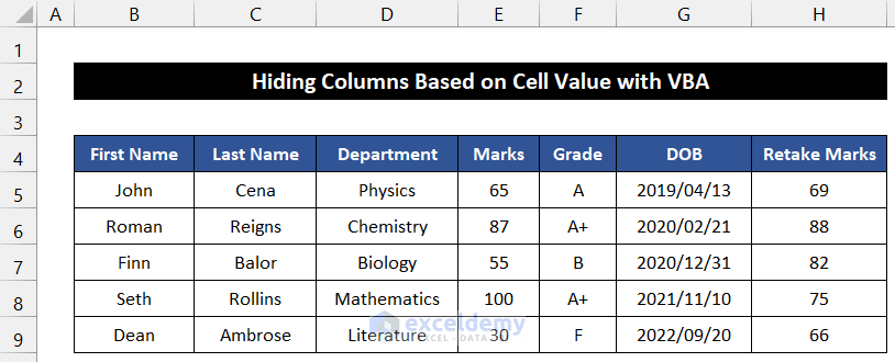
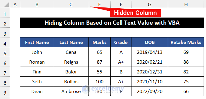
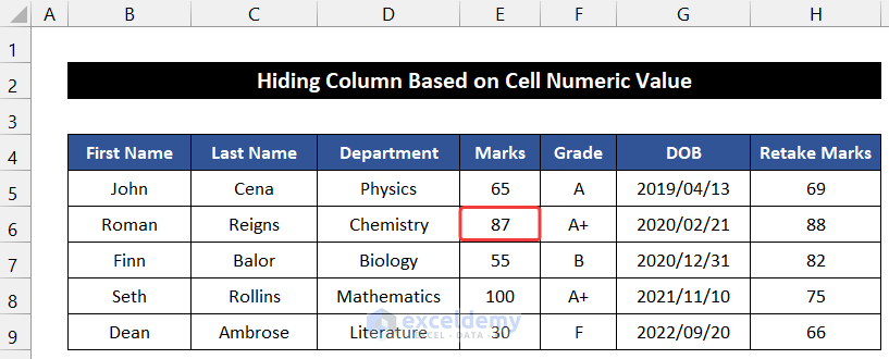
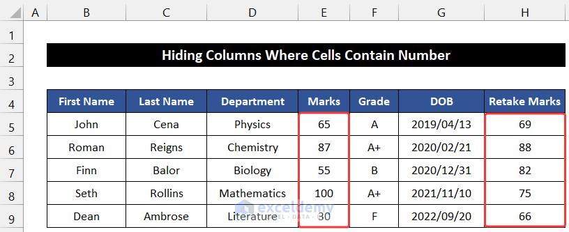
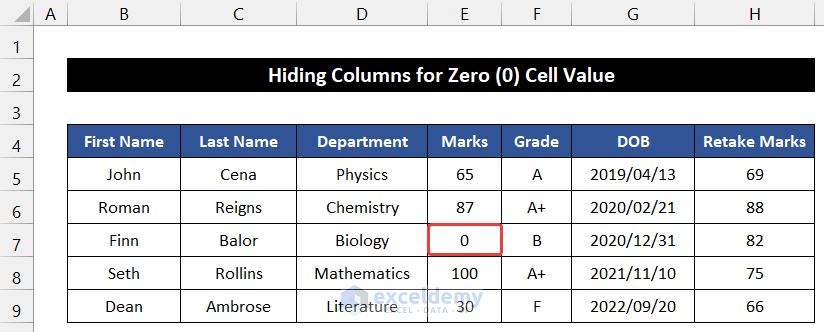
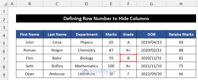
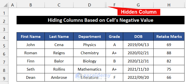
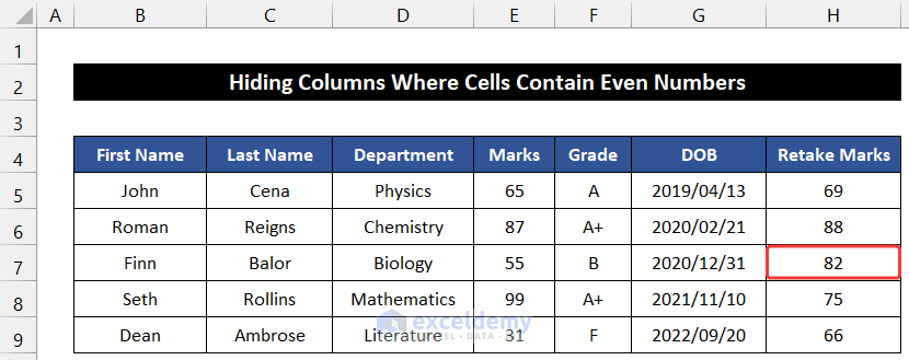
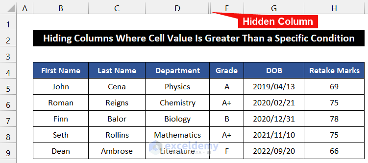
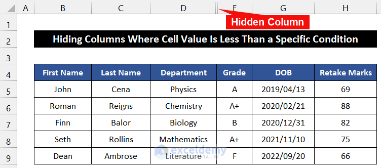
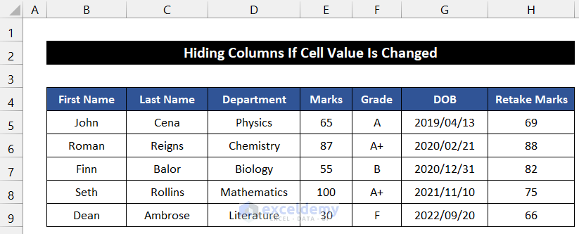
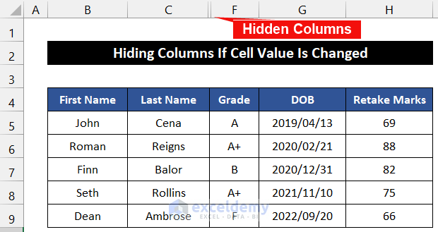
How to Use Excel VBA to Hide Columns Based on Cell Value (15 Examples)

To demonstrate, we have a dataset of 5 students. Their name, department, examination marks, grades, DOB, and retake examination marks are in the range of cells B5:H9. We will hide columns based on different cell value criteria in our examples.

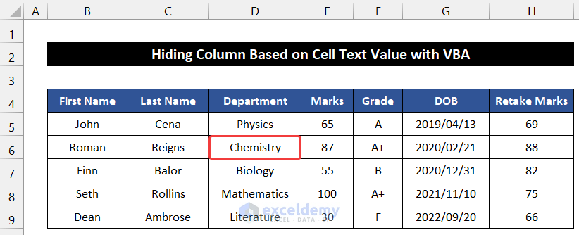
Method 1 – Hide Columns Based on Cell Text Value with VBA

Steps:

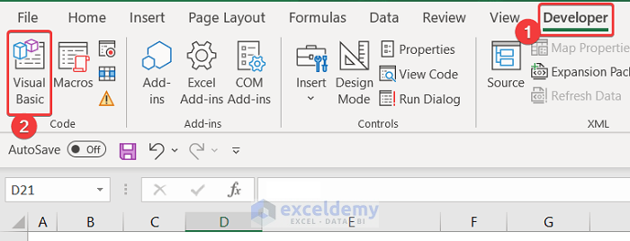
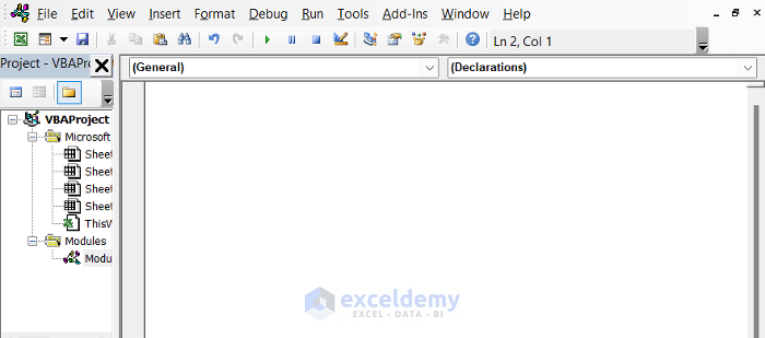
Go to the Developer tab and click on Visual Basic. If you don’t have that, you must enable the Developer tab. Or press ‘Alt+F11’ to open the Visual Basic Editor.

A dialog box will appear.
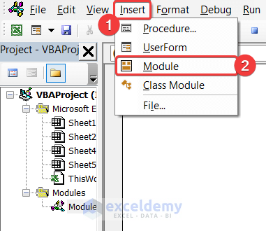
In the Insert tab on that box, click Module.

Enter the following visual code in that empty editor box.

Sub Hide_Columns_on_Cell_Text_Value()
    StartColumn = 2
    LastColumn = 10
    iRow = 6
    For i = StartColumn To LastColumn
        If Cells(iRow, i).Value <> "Chemistry" Then
        Cells(iRow, i).EntireColumn.Hidden = False
        Else
        Cells(iRow, i).EntireColumn.Hidden = True
        End If
    Next i
End Sub

Press ‘Ctrl+S’ to save the code.
Close the Editor tab.
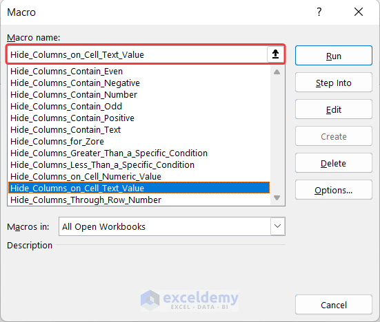
In the Developer tab, click on Macros, located in the group Code.

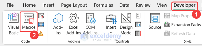
A new dialog box called Macro will appear. Select Hide_Columns_on_ Cell_Text_Value.
Click on the Run button to run this code.

You will see the column which contains the text Chemistry disappears from our dataset.

Breakdown of VBA Code

First, provide a name for the sub-procedure, which is Hide_Columns_on_Cell_ Text_Value.

Then, we declare the first and last columns of our dataset: StartColumn and LastColumn.

Moreover, we declare the row number through iRow where the text may exist.

After that, we used a VBA For Loop to check from the StartColumn to the LastColumn.

In addition, we used a conditional VBA IF ELSE loop to check our desired value in each cell.

Finally, the sub-procedure of the code.

Method 2 – Hide Column Based on Cell Numeric Value

Steps:

Go to the Developer tab and click on Visual Basic. If you don’t have that, you must enable the Developer tab. OR press ‘Alt+F11’ to open the Visual Basic Editor.

A dialog box will appear.
In the Insert tab on that box, click Module.

Enter the following visual code in that empty editor box.

Sub Hide_Columns_on_Cell_Numeric_Value()
    StartColumn = 2
    LastColumn = 8
    iRow = 6
    For i = StartColumn To LastColumn
        If Cells(iRow, i).Value <> "87" Then
        Cells(iRow, i).EntireColumn.Hidden = False
        Else
        Cells(iRow, i).EntireColumn.Hidden = True
        End If
    Next i
End Sub

Press ‘Ctrl+S’ to save the code.
Close the Editor tab.
In the Developer tab, click on Macros, located in the group Code.

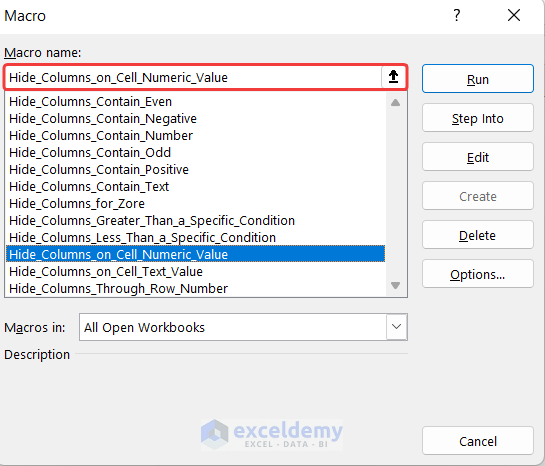
A new dialog box called Macro will appear.
Select Hide_Columns_on _Cell_Numeric_Value and click the Run button to run this code.

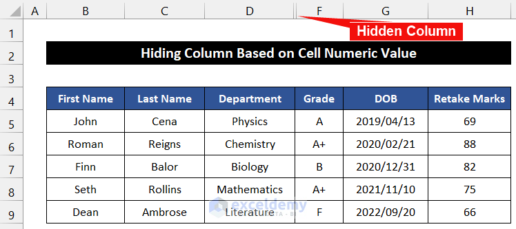
You will see a column containing 87, which is hidden from our dataset.

Breakdown of VBA Code

First, provide a name for the sub-procedure, which is Hide_Columns_on_Cell_ Numeric_Value.

Then, we declare the first and last columns of our dataset: StartColumn and LastColumn.

Moreover, we declare the row number through iRow where the number may exist.

After that, we used a VBA For Loop to check from the StartColumn to the LastColumn.

In addition, we used a conditional VBA IF ELSE loop to check our desired value in each cell.

Finally, end the sub-procedure of the code.

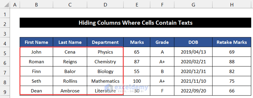
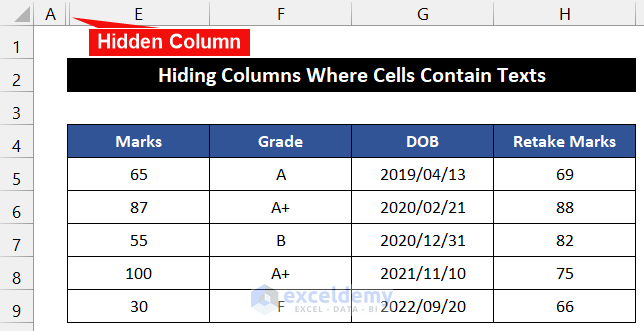
Method 3 – Hide Columns Where Cells Contain Texts

Steps:

Go to the Developer tab and click on Visual Basic. If you don’t have that, you must enable the Developer tab. OR press ‘Alt+F11’ to open the Visual Basic Editor.

A dialog box will appear.
In the Insert tab on that box, click Module.

Enter the following visual code in that empty editor box.

Sub Hide_Columns_Contain_Text()
    StartRow = 5
    LastRow = 9
    StartCol = 2
    LastCol = 8
    For i = StartRow To LastRow
        For j = StartCol To LastCol
        If IsNumeric(Cells(i, j)) = False Then
        Columns(j).EntireColumn.Hidden = True
        End If
        Next j
    Next i
End Sub

Press ‘Ctrl+S’ to save the code.
Close the Editor tab.
In the Developer tab, click on Macros, located in group Code.

A new dialog box called Macro will appear. Select Hide_Columns_ Contains_Text.
Click on the Run button to run this code.

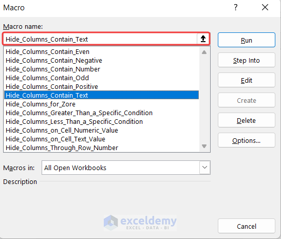
You will see all the columns that contain text disappear from our dataset.

Breakdown of VBA Code

First, provide a name for the sub-procedure, which is Hide_Columns_Contain_Text.

Then, we declare the first and last columns of our dataset: StartRow, LastRow, StartCol, and LastCol.

After that, we used a VBA For Loop to check from the StartRow to LastRow and StartCol to LastCol.

In addition, we used a conditional VBA IF ELSE loop to check our desired requirement in each cell.

Finally, end the sub-procedure of the code.

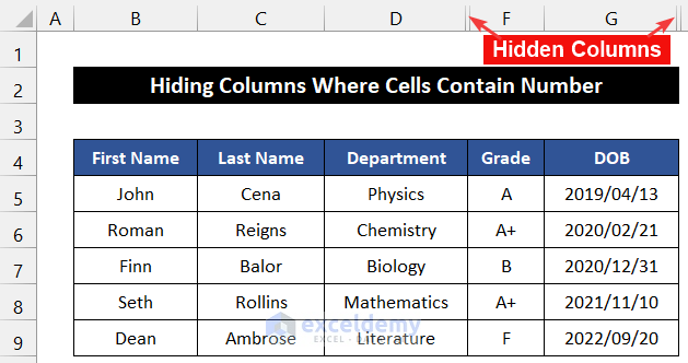
Method 4 – Hide Columns Where Cells Contain Number

Steps:

Go to the Developer tab and click on Visual Basic. If you don’t have that, you must enable the Developer tab. OR press ‘Alt+F11’ to open the Visual Basic Editor.

A dialog box will appear.
In the Insert tab on that box, click Module.

Enter the following visual code in that empty editor box.

Sub Hide_Columns_Contain_Number()
    StartRow = 5
    LastRow = 9
    StartCol = 2
    LastCol = 8
    For i = StartRow To LastRow
        For j = StartCol To LastCol
        If IsNumeric(Cells(i, j)) = True Then
        Columns(j).EntireColumn.Hidden = True
        End If
        Next j
    Next i
End Sub

Press ‘Ctrl+S’ to save the code.
Close the Editor tab.
In the Developer tab, click on Macros, located in group Code.

A new dialog box called Macro will appear.
Select Hide_All_Columns_Contain_Number and click on the Run button to run this code.

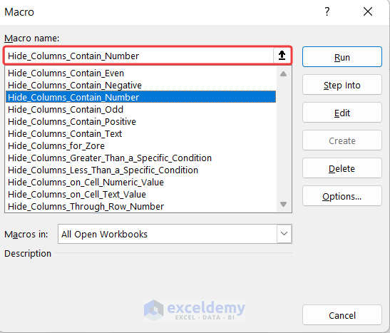
You will see all the columns which contain the numeric values disappear from our dataset.

Breakdown of VBA Code

First, provide a name for the sub-procedure, which is Hide_Columns_Contain _Number.

Then, we declare the first and last columns of our dataset: StartRow, LastRow, StartCol, and LastCol.

After that, we used a VBA For Loop to check from the StartRow to LastRow and StartCol to LastCol.

In addition, we used a conditional VBA IF ELSE loop to check our desired requirement in each cell.

Finally, end the sub-procedure of the code.

Method 5 – Hide Columns for Zero (0) Cell Value

Steps:

Go to the Developer tab and click on Visual Basic. If you don’t have that, you must enable the Developer tab. OR press ‘Alt+F11’ to open the Visual Basic Editor.

A dialog box will appear.
In the Insert tab on that box, click Module.

Enter the following visual code in that empty editor box.

Sub Hide_Columns_for_Zero()
    StartColumn = 2
    LastColumn = 8
    iRow = 7
    For i = StartColumn To LastColumn
        If Cells(iRow, i).Value <> "0" Then
        Cells(iRow, i).EntireColumn.Hidden = False
        Else
        Cells(iRow, i).EntireColumn.Hidden = True
        End If
    Next i
End Sub

Press ‘Ctrl+S’ to save the code.
Close the Editor tab.
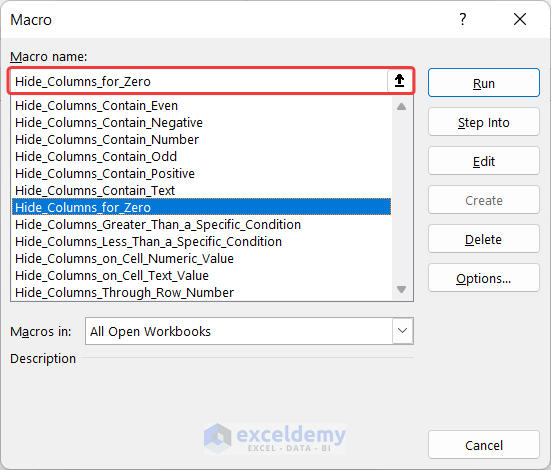
In the Developer tab, click on Macros, located in group Code.

A new dialog box called Macro will appear. Select Hide_Columns_for _Zore.
Click on the Run button to run this code.

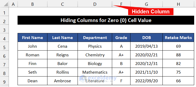
You will see the column that contains the Zero (0) values hidden from our dataset.

Breakdown of VBA Code

First, provide a name for the sub-procedure, which is Hide_Columns_for_Zore.

Then, we declare the first and last columns of our dataset: StartColumn and LastColumn.

Moreover, we declare the row number through iRow where the number may exist.

After that, we used a VBA For Loop to check from the StartColumn to the LastColumn.

In addition, we used a conditional VBA IF ELSE loop to check the Zero (0) value in each cell.

Finally, end the sub-procedure of the code.

Method 6 – Defining a Row Number to Hide Columns

Steps:

Go to the Developer tab and click on Visual Basic. If you don’t have that, you must enable the Developer tab. OR press ‘Alt+F11’ to open the Visual Basic Editor.

A dialog box will appear.
In the Insert tab on that box, click Module.

Enter the following visual code in that empty editor box.

Sub Hide_Columns_Through_Row_Number()
Dim A As Range
    For Each A In ActiveWorkbook.ActiveSheet.Rows("7").Cells
        If A.Value = "B" Then
        A.EntireColumn.Hidden = True
        End If
    Next A
End Sub

Press ‘Ctrl+S’ to save the code.
Close the Editor tab.
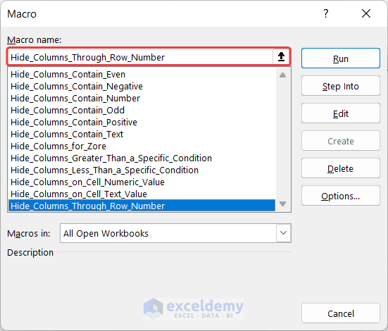
In the Developer tab, click on Macros, located in group Code.

A new dialog box called Macro will appear. Select Hide_Columns_ Through_Row_Number.
Click on the Run button to run this code.

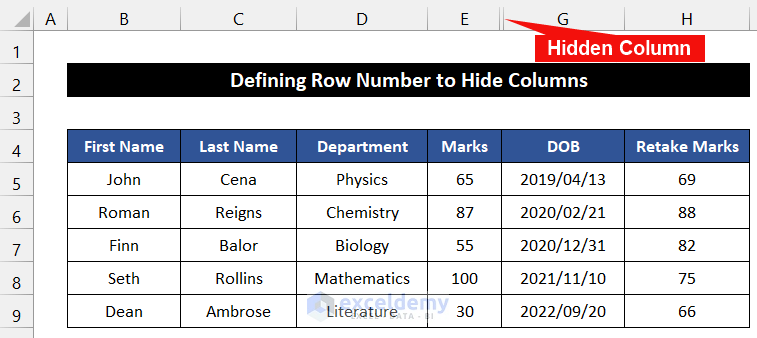
You will see the column that contains our chosen B character disappears from our dataset.

Breakdown of VBA Code

First, provide a name for the sub-procedure, which is Hide_Columns_Through_Row_ Number.

Then, we declare a variable.

After that, we used a VBA For Loop, where we mentioned the row number.

In addition, we used a conditional VBA IF ELSE loop to check the cell value B in each cell.

Finally, end the sub-procedure of the code.

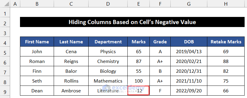
Method 7 – Hide Columns Based on Cell’s Negative Value

Steps:

Go to the Developer tab and click on Visual Basic. If you don’t have that, you must enable the Developer tab. OR press ‘Alt+F11’ to open the Visual Basic Editor.

A dialog box will appear.
In the Insert tab on that box, click Module.

Enter the following visual code in that empty editor box.

Sub Hide_Columns_Contain_Negative()
   StartColumn = 2
    LastColumn = 8
    iRow = 9
    For i = StartColumn To LastColumn
        If Cells(iRow, i).Value < "0" Then
        Cells(iRow, i).EntireColumn.Hidden = True
        Else
        Cells(iRow, i).EntireColumn.Hidden = False
        End If
    Next i
End Sub

Press ‘Ctrl+S’ to save the code.
Close the Editor tab.
In the Developer tab, click on Macros, located in group Code.

A new dialog box called Macro will appear. Select Hide_Columns_Contain _Negative.
Click on the Run button to run this code.

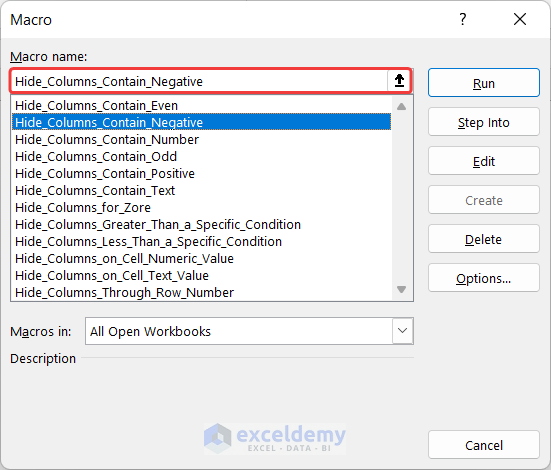
You will see the column that contains the negative value disappears from our dataset.

Breakdown of VBA Code

First, provide a name for the sub-procedure, which is Hide_Columns_Contain_ Negative.

Then, we declare the first and last columns of our dataset: StartColumn and LastColumn.

Moreover, we declare the row number through iRow where the number may exist.

After that, we used a VBA For Loop to check from the StartColumn to the LastColumn.

In addition, we used a conditional VBA IF ELSE loop to check the value less than Zero (0) or a negative number in each cell.

Finally, end the sub-procedure of the code.

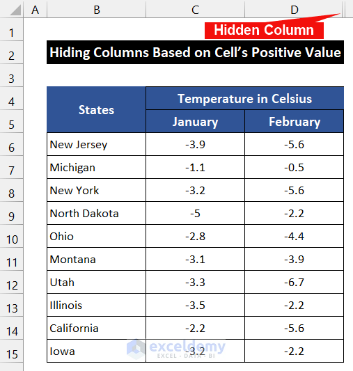
Method 8 – Hide Columns Based on Cell’s Positive Value

Steps:

Go to the Developer tab and click on Visual Basic. If you don’t have that, you must enable the Developer tab. OR press ‘Alt+F11’ to open the Visual Basic Editor.

A dialog box will appear.
In the Insert tab on that box, click Module.

Enter the following visual code in that empty editor box.

Sub Hide_Columns_Contain_Positive()
    StartRow = 5
    LastRow = 9
    StartCol = 2
    LastCol = 8
    For i = StartRow To LastRow
        For j = StartCol To LastCol
        If IsNumeric(Cells(i, j)) = True Then
            If Cells(i, j).Value > 0 Then
            Columns(j).EntireColumn.Hidden = True
            End If
        End If
        Next j
    Next i
End Sub

Press ‘Ctrl+S’ to save the code.
Close the Editor tab.
In the Developer tab, click on Macros, located in group Code.

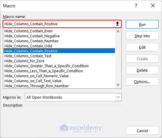
A new dialog box called Macro will appear. Select Hide_Columns_Contain _Positive.
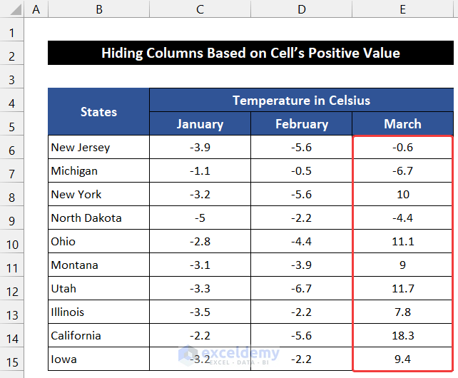
Click on the Run button to run this code.

You will see the column that contains the negative value disappears from our dataset.

Breakdown of VBA Code

First, provide a name for the sub-procedure, which is Hide_Columns_Contain_ Positive.

Then, we declare the first and last columns of our dataset: StartRow, LastRow, StartCol, and LastCol.

After that, we used a VBA For Loop to check from the StartRow to LastRow and StartCol to LastCol.

In addition, we used a conditional VBA IF ELSE loop to check the positive value in each cell.

Finally, end the sub-procedure of the code.

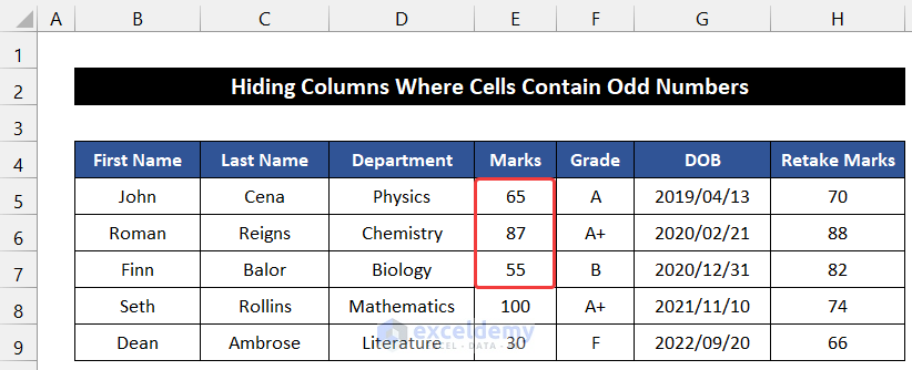
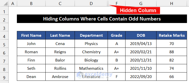
Method 9 – Applying a Macro to Hide Columns Where Cells Contain Odd Numbers

Steps:

Go to the Developer tab and click on Visual Basic. If you don’t have that, you must enable the Developer tab. OR press ‘Alt+F11’ to open the Visual Basic Editor.

A dialog box will appear.
In the Insert tab on that box, click Module.

Enter the following visual code in that empty editor box.

Sub Hide_Columns_Contain_Odd()
    StartRow = 5
    LastRow = 9
    StartCol = 2
    LastCol = 8
    For i = StartRow To LastRow
        For j = StartCol To LastCol
        If IsNumeric(Cells(i, j)) = True Then
            If Cells(i, j).Value Mod 2 = 1 Then
            Columns(j).EntireColumn.Hidden = True
            End If
        End If
        Next j
    Next i
End Sub

Press ‘Ctrl+S’ to save the code.
Close the Editor tab.
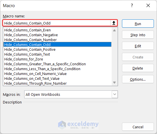
In the Developer tab, click on Macros, located in group Code.

A new dialog box called Macro will appear. Select Hide_Columns_Contain_Odd.
Cclick on the Run button to run this code.

You will see column E disappears from our dataset.

Breakdown of VBA Code

First, provide a name for the sub-procedure, which is Hide_Columns_Contain_Odd.

Then, we declare the first and last columns of our dataset: StartRow, LastRow, StartCol, and LastCol.

After that, we used a VBA For Loop to check from the StartRow to LastRow and StartCol to LastCol.

In addition, we used a conditional VBA IF ELSE loop to check whether the value is odd or even in each cell.

Finally, end the sub-procedure of the code.

Method 10 – Apply a Macro to Hide Columns Where Cells Contain Even Numbers

Steps:

Go to the Developer tab and click on Visual Basic. If you don’t have that, you must enable the Developer tab. OR press ‘Alt+F11’ to open the Visual Basic Editor.

A dialog box will appear.
In the Insert tab on that box, click Module.

Enter the following visual code in that empty editor box.

Sub Hide_Columns_Contain_Even()
    StartRow = 5
    LastRow = 9
    StartCol = 2
    LastCol = 8
    For i = StartRow To LastRow
        For j = StartCol To LastCol
        If IsNumeric(Cells(i, j)) = True Then
            If Cells(i, j).Value Mod 2 = 0 Then
            Columns(j).EntireColumn.Hidden = True
            End If
        End If
        Next j
    Next i
End Sub

Press ‘Ctrl+S’ to save the code.
Close the Editor tab.
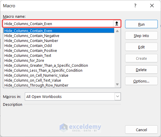
In the Developer tab, click on Macros, located in group Code.

A new dialog box called Macro will appear. Select Hide_Columns_Contain_Even.
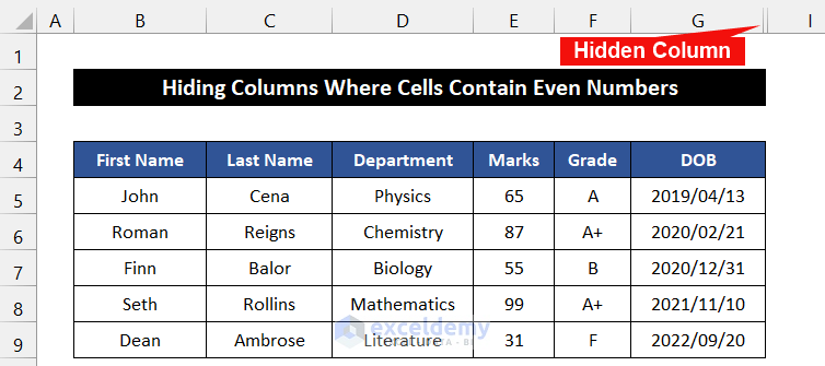
Click on the Run button to run this code.

You will see column H disappear from our dataset.

Breakdown of VBA Code

First, provide a name for the sub-procedure, which is Hide_Columns_Contain_Even.

Then, we declare the first and last columns of our dataset: StartRow, LastRow, StartCol, and LastCol.

After that, we used a VBA For Loop to check from the StartRow to LastRow and StartCol to LastCol.

In addition, we used a conditional VBA IF ELSE loop to check whether the value is odd or even in each cell.

Finally, end the sub-procedure of the code.

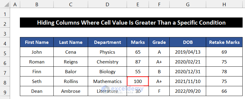
Method 11 – Hiding Columns Where a Cell Value Is Greater Than a Specific Condition

Steps:

G to the Developer tab and click on Visual Basic. If you don’t have that, you must enable the Developer tab. OR press ‘Alt+F11’ to open the Visual Basic Editor.

A dialog box will appear.
In the Insert tab on that box, click Module.

Enter the following visual code in that empty editor box.

Sub Hide_Columns_Greater_Than_a_Specific_Condition()
    StartRow = 5
    LastRow = 9
    StartCol = 2
    LastCol = 8
    For i = StartRow To LastRow
        For j = StartCol To LastCol
        If IsNumeric(Cells(i, j)) = True Then
            If Cells(i, j).Value > 90 Then
            Columns(j).EntireColumn.Hidden = True
            End If
        End If
        Next j
    Next i
End Sub

Press ‘Ctrl+S’ to save the code.
Close the Editor tab.
In the Developer tab, click on Macros, located in group Code.

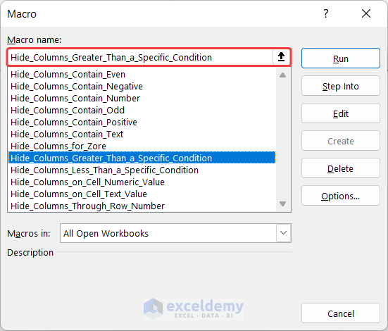
A new dialog box called Macro will appear.
Select Hide_Columns_Greater_Than_a_Specific_Condition and click on the Run button to run this code.

You will see column E disappears from our dataset.

Breakdown of VBA Code

First, provide a name for the sub-procedure, which is Hide_Columns_Greater_ Than_a_Specific_Condition.

Then, we declare the first and last columns of our dataset: StartRow, LastRow, StartCol, and LastCol.

After that, we used a VBA For Loop to check from the StartRow to LastRow and StartCol to LastCol.

In addition, we used a conditional VBA IF ELSE loop to check whether the value is greater than 90 in each cell.

Finally, end the sub-procedure of the code.

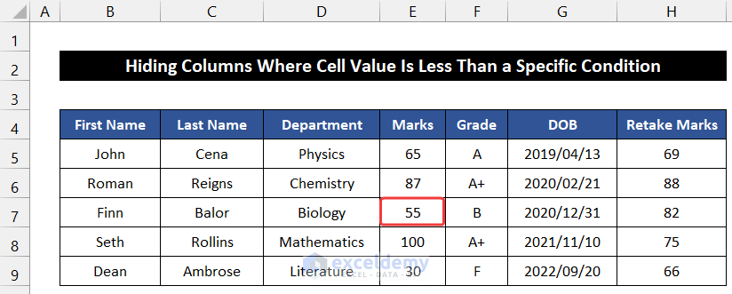
Method 12 – Hide Columns Where a Cell Value Is Less Than a Specific Condition

Steps:

Go to the Developer tab and click on Visual Basic. If you don’t have that, you must enable the Developer tab. OR press ‘Alt+F11’ to open the Visual Basic Editor.

A dialog box will appear.
In the Insert tab on that box, click Module.

Enter the following visual code in that empty editor box.

Sub Hide_Columns_Less_Than_a_Specific_Condition()
    StartRow = 5
    LastRow = 9
    StartCol = 2
    LastCol = 8
    For i = StartRow To LastRow
        For j = StartCol To LastCol
        If IsNumeric(Cells(i, j)) = True Then
            If Cells(i, j).Value < 60 Then
            Columns(j).EntireColumn.Hidden = True
            End If
        End If
        Next j
    Next i
End Sub

Press ‘Ctrl+S’ to save the code.
Close the Editor tab.
In the Developer tab, click on Macros, located in group Code.

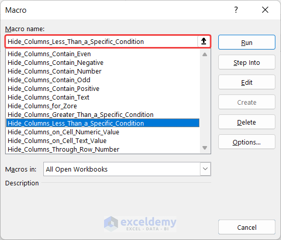
A new dialog box called Macro will appear.
Select Hide_Columns_Less_Than_a_Specific_Condition and click on the Run button to run this code.

You will see column E disappears from our dataset.

Breakdown of VBA Code

First, provide a name for the sub-procedure, which is Hide_Columns_Less _Than_a_Specific_Condition.

Then, we declare the first and last columns of our dataset: StartRow, LastRow, StartCol, and LastCol.

After that, we used a VBA For Loop to check from the StartRow to LastRow and StartCol to LastCol.

In addition, we used a conditional VBA IF ELSE loop to check whether the value is less than 60 in each cell.

Finally, end the sub-procedure of the code.

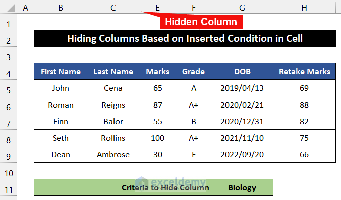
Method 13 – Hide Columns Based on Inserted Conditions in a Cell

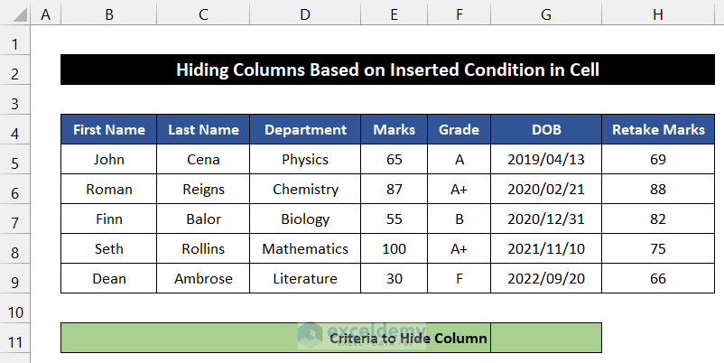
Step:

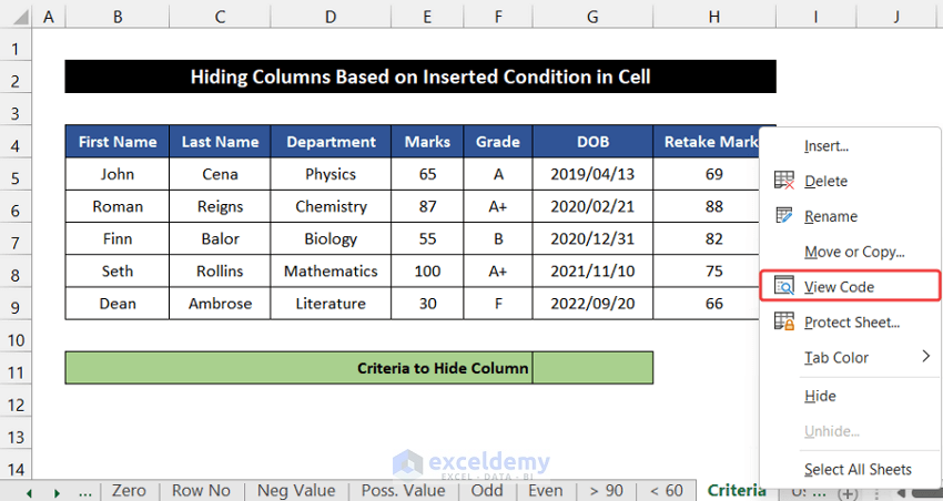
Right-click on the sheet name in the Sheet Name Bar.
The Context Menu will appear.
Select the View Code option.

A white dialog box will appear.
Enter the following visual code in that empty editor box.

Private Sub Worksheet_SelectionChange(ByVal Target As Range)
    StartColumn = 2
    LastColumn = 8
    iRow = 7
    For i = StartColumn To LastColumn
        If Cells(iRow, i).Value = Range("G11").Value Then
            Cells(iRow, i).EntireColumn.Hidden = True
    Else
        Cells(iRow, i).EntireColumn.Hidden = False
        End If
    Next i
End Sub

Press ‘Ctrl+S’ to save the code.
After that, close the Editor tab.
You don’t have to run this code. When you will save the code, it will run automatically.
If you enter text or numbers that exist in the dataset, you will see that the column will disappear. To demonstrate it, we entered Biology, and pressed Enter.

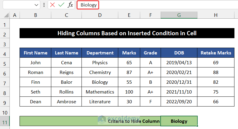
You will notice that column D will disappear.

Breakdown of VBA Code

First, initiating an event under the specific worksheet where Target is passed as an argument with Range type. When the Range changes, the event occurs.

Then, we declare the first and last columns of our dataset: StartColumn and LastColumn.

Moreover, we declare the row number through iRow where the text may exist.

After that, we used a VBA For Loop to check from the StartColumn to the LastColumn.

We used a conditional VBA IF ELSE loop to check our desired value in each cell. In addition, we also mentioned the input cell range.

Finally, end the sub-procedure of the code.

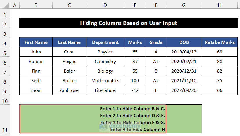
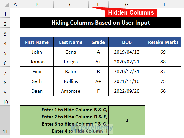
Method 14 – Hide Columns Based on User Input

Step:

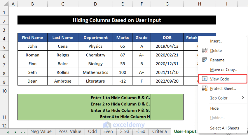
Right-click on the sheet name in the Sheet Name Bar.
The Context Menu will appear.
Select the View Code option.

A white dialog box will appear.
Enter the following visual code in that empty editor box.

Private Sub Worksheet_SelectionChange(ByVal Target As Range)
i = Range("G11").Value
Select Case i
Case 1: Columns("B:C").EntireColumn.Hidden = False
Columns("B:C").EntireColumn.Hidden = True
Case 2: Columns("D:E").EntireColumn.Hidden = False
Columns("D:E").EntireColumn.Hidden = True
Case 3: Columns("F:G").EntireColumn.Hidden = False
Columns("F:G").EntireColumn.Hidden = True
Case 4: Columns("H:I").EntireColumn.Hidden = False
Columns("H:I").EntireColumn.Hidden = True
Case Else
Columns("B:I").EntireColumn.Hidden = False
End Select
End Sub

Press ‘Ctrl+S’ to save the code.
Close the Editor tab.
In this case, you don’t have to run this code. When you save it, it will run automatically.
Now, If you input a number according to the list, you will see that two columns will disappear. To demonstrate, we entered 2 and pressed Enter.

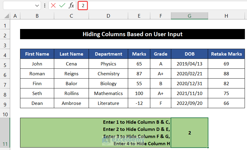
You will notice columns D and E disappear.

Hence, we can say that our visual code worked precisely, and we are able to apply Excel VBA to hide columns based on cell value.

Breakdown of VBA Code

First, initiating an event under the specific worksheet where Target is passed as an argument with Range type. When the Range changes, the event occurs.

Then, we declare the cell range where the user inputs the value.

We used a conditional VBA IF ELSE loop to check for each user input and show the result.

Finally, end the sub-procedure of the code.

Method 15 – Hide Columns If a Cell Value Is Changed

Step:

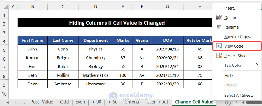
Right-click on the sheet name in the Sheet Name Bar.
The Context Menu will appear.
Select the View Code option.

A white dialog box will appear.
Enter he following visual code in that empty editor box.

Option Explicit
Private Sub Worksheet_Change(ByVal Target As Range)
    Dim iCell As Range: Set iCell = Me.Range("D5")
    If Intersect(iCell, Target) Is Nothing Then Exit Sub
    If IsNumeric(iCell.Value) Then
        RowHide iCell
    End If
End Sub
Sub RowHide(ByVal SourceCell As Range)
    If SourceCell.Value = 0 Then
        SourceCell.Worksheet.Columns("D:E").Hidden = True
    Else
        SourceCell.Worksheet.Columns("D:E").Hidden = False
    End If
End Sub

Press ‘Ctrl+S’ to save the code.
Close the Editor tab.
You don’t have to run this code. When you will save the code, it will run automatically.
If you change the cell value in cell D5 from Physics to 0, press Enter.

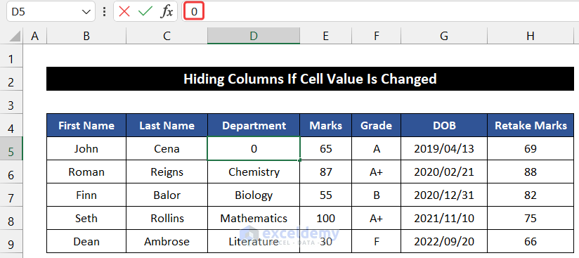
You will see that columns D and E will disappear.

Breakdown of VBA Code

First, we were forced to declare all variables.

Then, initiating an event under the specific worksheet where Target passed as an argument with Range type. When the Range changes, the event occurs.

After that, we declared where we would change the value.

End the first sub-procedure.

Next, Initiate the sub-procedure of the ColumnHide macro. Variable SourceCell passed as a Range type argument.

We used a conditional VBA IF ELSE loop to hide columns “D:E” if the Zero (0) value is imputed in cell D5.

Finally, end the sub-procedure of the code.

Download the Practice Workbook

Download this workbook for practice.

Hide Columns Based on Cell Value.xlsm

How to Unhide All Columns with Excel VBA

Get FREE Advanced Excel Exercises with Solutions!

How to Use Excel VBA to Hide Columns Based on Cell Value (15 Examples)

Method 1 – Hide Columns Based on Cell Text Value with VBA

Method 2 – Hide Column Based on Cell Numeric Value

Method 3 – Hide Columns Where Cells Contain Texts

Method 4 – Hide Columns Where Cells Contain Number

Method 5 – Hide Columns for Zero (0) Cell Value

Method 6 – Defining a Row Number to Hide Columns

Method 7 – Hide Columns Based on Cell’s Negative Value

Method 8 – Hide Columns Based on Cell’s Positive Value

Method 9 – Applying a Macro to Hide Columns Where Cells Contain Odd Numbers

Method 10 – Apply a Macro to Hide Columns Where Cells Contain Even Numbers

Method 11 – Hiding Columns Where a Cell Value Is Greater Than a Specific Condition

Method 12 – Hide Columns Where a Cell Value Is Less Than a Specific Condition

Method 13 – Hide Columns Based on Inserted Conditions in a Cell

Method 14 – Hide Columns Based on User Input

Method 15 – Hide Columns If a Cell Value Is Changed

Related Article

Leave a reply Cancel reply