Latest Posts From Md. Abdur Rahim Rasel

The WeekdayName function in Microsoft Excel returns a string that represents the day of the week when given a number between 1 and 7. The WeekdayName function ...

The Int function in Microsoft Excel returns the integer part of a value. The VBA Int is a built-in function in Excel. In Excel, it can be used as a worksheet ...

Method 1 - Applying the Refresh All Command to Refresh All Pivot Tables in Excel Step 1: Look at the pivot tables; the Grand Total of the Revenue Earned ...
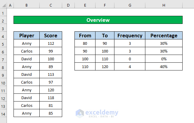
A percent frequency distribution can help you figure out what proportion of the distribution is made up of specific values. By grouping values together, a ...
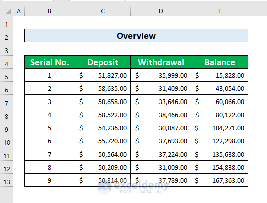
Consider the following dataset of cash flow inside some bank accounts. The deposits and withdrawals are listed in columns C and D. We’ll calculate their ...

The Trim Function can trim extra leading and trailing spaces within text cells in Excel. Normally, the spaces given before a word are called leading spaces. ...
Method 1 - Apply the Keyboard Shortcuts to AutoFit in Excel In our dataset, we can apply AutoFit by using the keyboard shortcuts in two ways. The first one is ...

Excel allows you to easily format cells in a spreadsheet. Formatting options like font, font size, text alignment, cell borders, background fills and more ...
We have a dataset where some Project Names and their Starting Date and Total Days to complete these Projects are given in Column B, Column C, and Column D, ...

Let’s say there's a dataset where different types of Fruits and their prices in January are given in Column B and Column C, respectively. You need to find the ...

In real life, statistical calculation is our quotidian work. By using Microsoft Excel, we can easily perform these statistical calculations. The NORMINV ...

In this article, we’ll demonstrate various examples of how to use the WEEKNUM function effectively in Excel. Introduction to the WEEKNUM Function in ...

This is an overview: The YEARFRAC Function in Excel Function Objective The YEARFRAC function is used to calculate the fraction of the year ...

While working in Excel, sometimes we need to add or Shift a Row or Column in our Worksheet. When we insert a new Cell, it pushes the next cell up to the end of ...
Let's assume we have a dataset with First Names, Last Names, Salaries, and Countries in Columns B, C, E, and D respectively. Method 1 - Applying the ...
See Our Reviews at


Hello RAVI
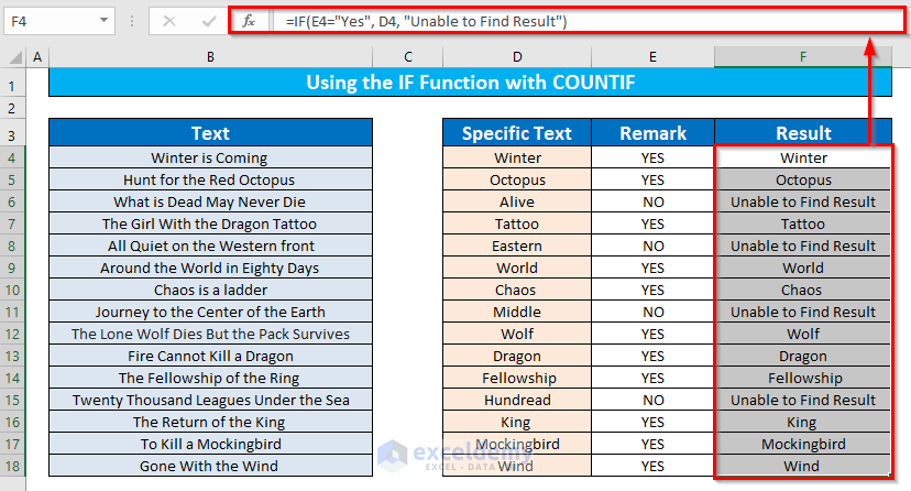
Thank you for your comment. When you are identifying the specific text from a string using Excel formulas, the specific text is known by you. So, I think if the return of the Excel formulas is TRUE you will be able to identify that specific text otherwise it returns FALSE. That’s why I think the above formula is appropriate to find out the specific text from a string. According to your question, I will introduce you to an efficient Excel function named the IF function to get the specific text. The IF function is,
=IF(E4=”YES”,D4,”Unable to Find Result”)Look at the below screenshot.
For the convenience of your work, please download the below Excel file which is provided by Exceldemy:
https://www.exceldemy.com/wp-content/uploads/2022/08/Excel-If-Range-of-Cells-Contains-Specific-Text.xlsx
If the answer doesn’t fulfill your query, feel free to comment. Our Exceldemy Team is always there to help.
Hello MARK,
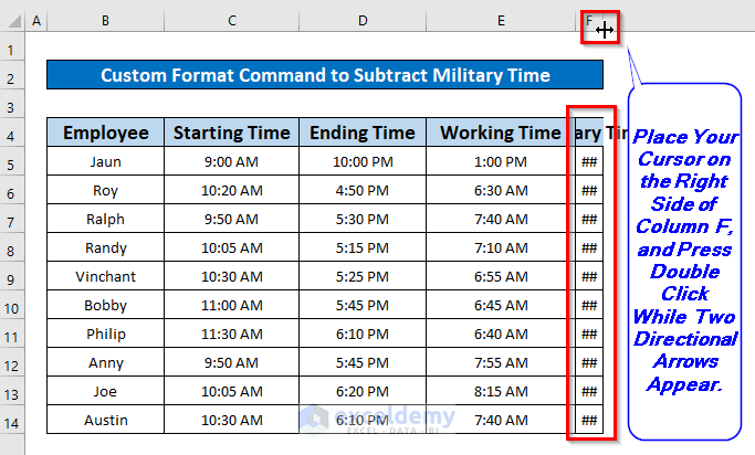
To solve your ###### issue in the calculation field simply AutoFit the column width. You can AutoFit the column width like below screenshot.
Thank you for your comment.
Hello JACK,
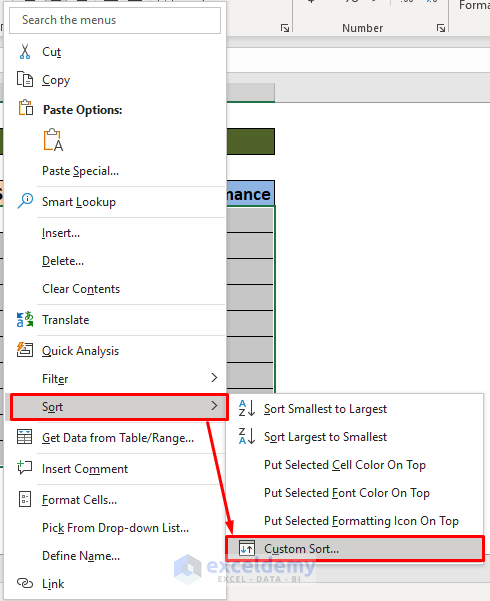
You can easily do that using the Custom Sort command. Let’s follow the instructions below:
Let’s Sales volumes less than 40 are marked with low performance. Sales volumes greater than 40 but less than 60 are marked with medium performance. Sales volumes greater than 60 are marked with high performance.
First of all, select cells range E5 to F14, and press right-click. As a result, a window pops up. From that window select Custom Sort under the Sort option.
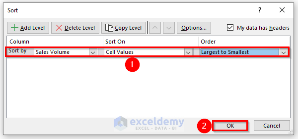
After that, do like the below screenshot.
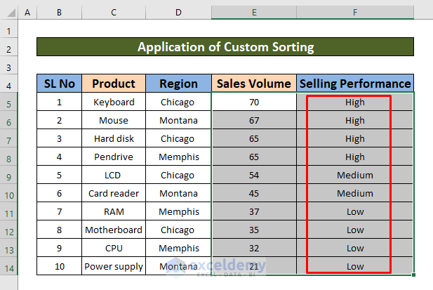
Finally, you will get your desired output.
Please download the below Excel file for your practice.
https://www.exceldemy.com/wp-content/uploads/2022/08/Advanced-Sorting-Options.xlsx
Thank you for your comment.
Regards
Md. Abdur Rahim Rasel(Exceldemy Team)
Hi TERRY MUNDY!
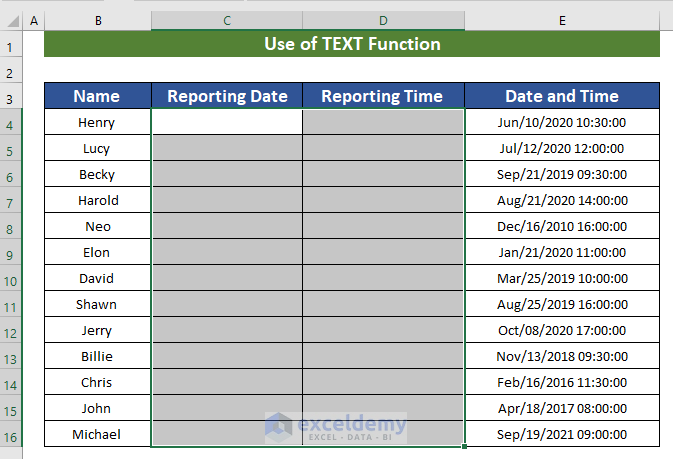
You can easily make the output cell permanent through you will delete the original Date and Time cells. First of all, use Ctrl + C on your keyboard to copy the output cell. Hence, use the paste special features to paste the value only from your Home ribbon. After that, you can delete the original Date and Time cells, the output cell will become permanent. Look at the below screenshot.
Thank you for your question.
Regards
Md. Abdur Rahim Rasel (Exceldemy Team)
Hi AHMAD KHAN!
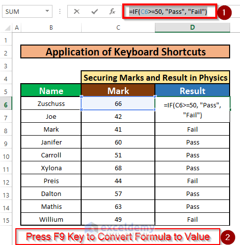
This article is how to Convert Formula to Value Without Paste Special in Excel. You can convert Formula in Value using the Keyboard shortcuts(F9), Right-Click Drag Down Option, Notepad to Convert Formula in Value, VBA code, Power Query, and so on. One suitable example is given below regarding your questions.
Suppose we have a data set that contains securing marks and results on Physics of several students of XYZ school. If a student secures less than 50, his/her result will Fail, and more than or equal to 50, his/her result will Pass. We will apply the IF function to do that. Let’s follow the instructions below.
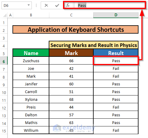
First of all, select the formula in the Formula bar, then press F9.
As a result, you will be able to convert the formula to value without paste special.
Please repeat the procedure for the rest of the cells in column D.
Please download the Excel file for your practice.
https://www.exceldemy.com/wp-content/uploads/2022/09/Convert-Formula-to-Value-Without-Paste-Special.xlsx
Thank you for your comment.
Personal Email for sending your Excel sheet: [email protected]
Regards
Md. Abdur Rahim Rasel (Exceldemy Team)
Hi AHMAD!
I have checked all of the solutions of the above article again that can figure out how to make the mouse scroll in excel. I think the article is appropriate to solve the vertical scroll not working problem in Excel. You can disable the Automatically hide scroll bars in the windows option in windows 11 pro from the setting option under the start menu bar.
Thank you for your comment.
If you cannot solve your problem, please mail me personally at below mail address.
[email protected]
Regards
Md. Abdur Rahim Rasel (Exceldemy Team)
Hello VADAKKUS!
To get the Stocks of the Indian Index instead of the NASDAQ Index, please use the below link in Method 3. The link is: https://www.moneycontrol.com/markets/indian-indices/
Thank you for your comment.
Regards
Md. Abdur Rahim Rasel (Exceldemy Team)
Hello BABA,
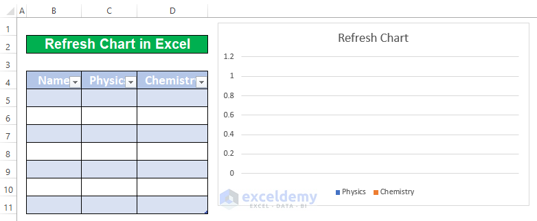
I have checked all of the methods of the above article again that can figure out how to refresh chart in excel. I think the article is appropriate to refresh chart in Excel. While removing data from the dataset, I would not get any error. Look at the below screenshot.
Thank you for your comment.
If you get error, please mail me personally at below mail address.
[email protected]
Regards
Md. Abdur Rahim Rasel (Exceldemy Team)
Hello, ROB!
Thanks for sharing your problem with us!
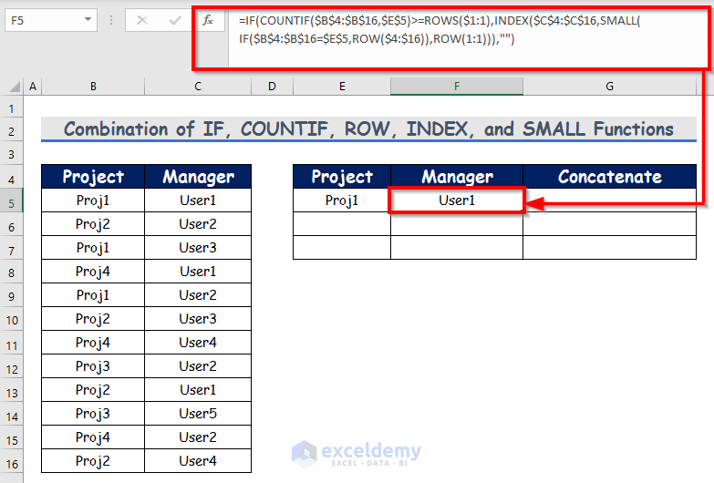
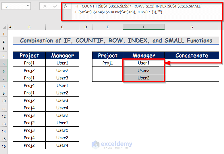
Let’s say, we have a dataset that contains several projects and project managers. You can know how many projects are shared among each pair of project managers by applying the IF, COUNTIF, ROW, INDEX, and SMALL functions. Hence, you can concatenate the projects with project managers using the Ampersand symbol.
Let’s follow the instructions below to solve your problem!
→ First of all, Select cell F5 and write down the below screenshot’s functions in that cell. Hence, press Enter on your keyboard to get your desired output.
=IF(COUNTIF($B$4:$B$16,$E$5)>=ROWS($1:1),INDEX($C$4:$C$16,SMALL(IF($B$4:$B$16=$E$5,ROW($4:$16)),ROW(1:1))),"")→ Further, AutoFill the functions to the rest of the cells in column F.
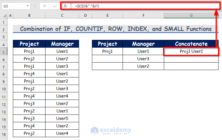
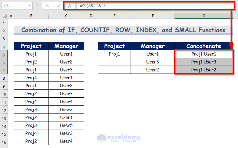
→ Now, we will concatenate a project and the project managers under that project. Insert the below formula into the formula bar.
=$E$5&" "&F5→ Hence, AutoFill the formula to the rest of the cells in column G.
Please download the Excel file for your practice.
https://www.exceldemy.com/wp-content/uploads/2022/10/COUNTIF-with-Multiple-Criteria.xlsx
Again Thank you for your comment.
Regards
Md. Abdur Rahim Rasel
Exceldemy Team
Hello KARTHIK!
Thanks for reaching out and sharing your problem with us.
I think the article will help you capture the data from pivot in the body of the mail as per the data range in a table format. Please read the article again.
If you are still facing issues, please mail us at the address below.
[email protected]
Again, thank you for being with us.
Regards
Md. Abdur Rahim Rasel
Exceldemy Team
Hello UMESH!
Thanks for reaching out and sharing your problem with us.
let’s break down the given formula =PRODUCT(SUM(B5:B14),SUM(C5:C14)) and provide a deeper interpretation:
SUM(B5:B14): calculates the sum of the values in the range from cell B5 to B14. It adds up all the numbers in that specified range.
SUM(C5:C14): calculates the sum of the values in the range from cell C5 to C14. It adds up all the numbers in that specified range.
=PRODUCT(SUM(B5:B14),SUM(C5:C14))
The outer PRODUCT function takes the results of the two SUM functions and multiplies them together. In other words, it multiplies the sum of values in range B5:B14 by the sum of values in range C5:C14.
When you AutoFill the above formula, it will automatically create relative cell references within a similar data range.
If you want to get the total product result in a single cell, use absolute cell references instead of relative cell references in the above formula. Then, use the following formula instead of the one above
=PRODUCT(SUM($B$5:$B$14),SUM($C$5:$C$14))
Again, thank you for being with us.
Regards
Md. Abdur Rahim Rasel
Exceldemy Team
Hello SAJJAD!
Thanks for reaching out and sharing your problem with us.
I think the article is appropriate for fixing your problem. You can try again following the steps in the article, and if you cannot fix the problem, feel free to ask for assistance.
Again, thank you for being with us.
Regards
Md. Abdur Rahim Rasel
Exceldemy Team
Dear Anton!
Thanks for reaching out and sharing your problem with us.
No, you can not set the color of negative numbers using hex values directly in the custom number format in Excel. The custom number format in Excel has predefined color names such as [Red], [Green], etc., but it doesn’t support specifying colors using hex values.
Again, thank you for being with us.
Regards
Md. Abdur Rahim Rasel
Exceldemy Team
Hello JAVIER!
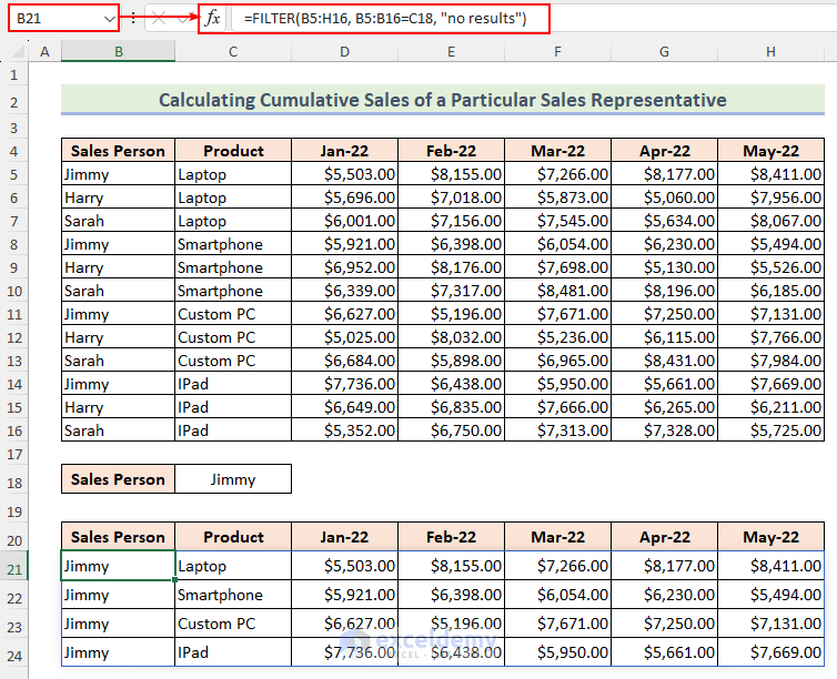
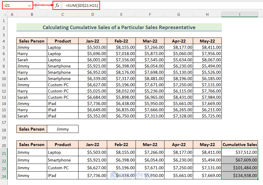
Thank you for sharing your problem with us. We have got a very simple solution to your problem. Let’s follow the instructions below to fix your problem.
In cell B21, write down the following FILTER function to filter Jimmy’s data.
=FILTER(B5:H16, B5:B16=C18, "no results")Hence, type the SUM function in cell I21 to calculate cumulative sales.
=SUM($D$21:H21)As a result, you will be able to calculate the cumulative sales of a particular sales representative.
Please download the Excel file for solving your problem and practice with it.
Cumulative Sales.xlsx
If you are still facing issues, please mail us at the address below.
[email protected]
Once again, thank you for your appreciation and for being with us.
Regards
Md. Abdur Rahim Rasel
Exceldemy Team
Hello PAUL!
Thanks for your feedback.
You can use the following VBA code to change “IsNumeric” to “IsText” for composing the text values instead of numeric values.
Please download the Excel file for solving your problem and practice with it.
Send Email Automatically.xlsm
If you are still facing issues, please mail us at the address below.
[email protected]
Again, thank you for being with us.
Regards
Md. Abdur Rahim Rasel
Exceldemy Team
Hello Shery!
Thanks for your feedback.
You can use the below VBA code to change the font and font size in the same cell range across all the sheets in the same workbook.
Please download the Excel file for solving your problem and practice with it.
Change Font Across All Sheets.xlsm
If you are still facing issues, please mail us at the address below.
[email protected]
Again, thank you for being with us.
Regards
Md. Abdur Rahim Rasel
Exceldemy Team
Hi MEAGAN!
You can set the below VBA code to send an email if D1>7 but also send an email if D5>2. The VBA code is:
Please download the Excel file for solving your problem and practice with it.
Automatically Send Emails from Excel Based on Cell Content.xlsm
If you cannot solve your problem, please mail us at the address below.
[email protected]
Thank you for being with us.
Regards
Md. Abdur Rahim Rasel
Exceldemy Team
Hello TOM DE JONGH!
Thanks for your query.
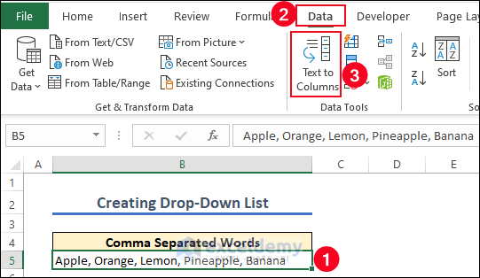
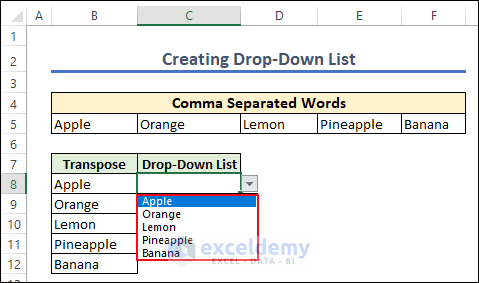
You have one cell with comma-separated words, and create a dropdown menu (list) from that, instead of creating a dropdown list from a column.
We will convert those comma-separated words into columns using the Text to Columns feature. Hence, transpose these words using the TRANSPOSE function. After that, we will create a drop-down list using the Data Validation feature.
Let’s follow the instructions below to learn!
To split the comma-separated words, go to,
Data >> Data Tools >> Text to Columns
We will use the comma as a delimiter.
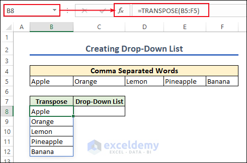
Hence, you will be able to split the comma-separated words and then in cell B8 apply the TRANSPOSE function to transpose row to column.
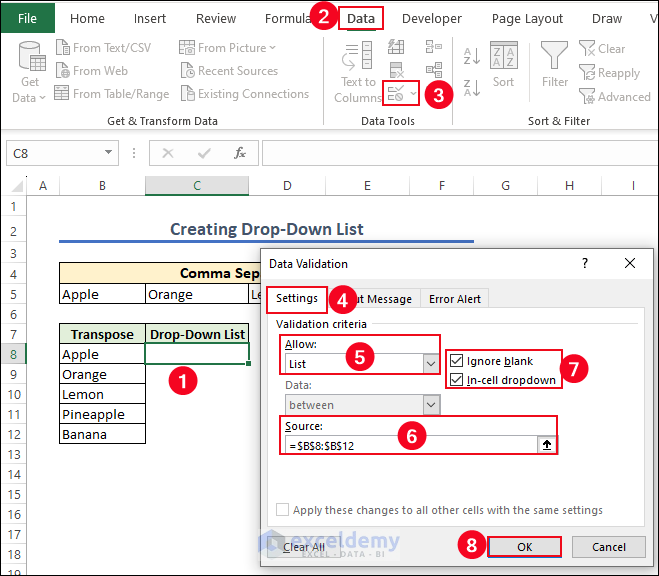
=TRANSPOSE(B5:F5)Now, we’ll select cell C8 to create the drop-down list using the Data Validation feature.
Finally, you will be able to create a drop-down menu from a comma-separated words cell.
Please download the Excel file to solve your problem and practice with it.
Creating Drop-Down List.xlsx
Now I think you can solve your problem. If you cannot solve your problem, you can contact with us via this mail [email protected]
Regards
Md. Abdur Rahim Rasel
Exceldemy Team
Hello IRINA!
Thanks for sharing your problem with us!
It would be better for us if you shared your Excel dataset to help us better understand your problem.
Don’t worry! I have created an Excel file to fix your problem. I have solved your problem based on the current working days. I have calculated the Progress of the work & the Estimated Days of the work (which represent the total days of working), and Working Days (the actual working days at that moment).
Please download the Excel file to solve your problem and practice with it.
Dates Calculation.xlsx
If you cannot solve your problem, please mail us at the address below.
[email protected]
You can also leave your problem on our Forum site.
Regards
Md. Abdur Rahim Rasel
Exceldemy Team
Hello ZAC!
Thanks for sharing your problem with us!
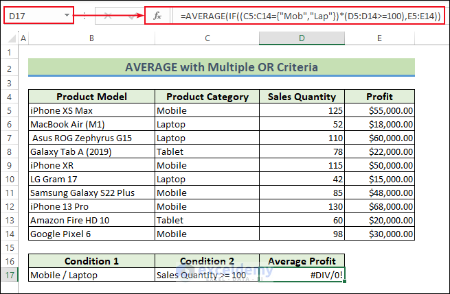
You’ve used the wording but could not find this last part anywhere else ‘Excel AVERAGE with Multiple OR Criteria in the Same Range’.
The formula returns #DIV/0! error because the matching values are different from the data table.
You can fix the issue using the following formula with a partial match.
Please download the Excel file for solving your problem and practice with it.
Excel AVERAGEIFS with Multiple Criteria in Same Range
If you cannot solve your problem, please mail us at the address below.
[email protected]
Regards
Md. Abdur Rahim Rasel
Exceldemy Team
Hi SANDEEP KOTHARI!
I have not encountered any problems while using MD. If you face any problems, please send us your Excel file.
Thank you for being with us.
Regards
Md. Abdur Rahim Rasel
Exceldemy Team
Hello, Robert Scott!
Thanks for sharing your problem with us!
We have checked the code and it’s working perfectly on our end. Here, we have set the date as
and 1 as the increment.
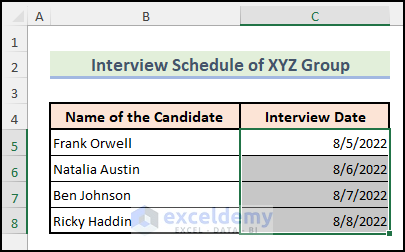
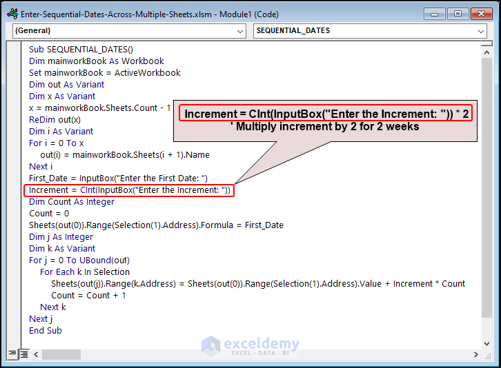
If you change the code as shown in the screenshot, the macro will increase the increment by 2 weeks. Otherwise, the macro will return the increment by 1 week.
If you cannot solve your problem, please mail us at the address below.
[email protected]
Regards
Md. Abdur Rahim Rasel (Exceldemy Team)
Hi TONY!
We checked the Excel file. It is working fine for an even and uneven amount of characters. Make sure the TRIM function and the text to the column are entered correctly. We suggest you download the file and practice there. If you are unable to solve your problem, you can also share your Excel file with us.
Thank you for being with us.
Regards
Md. Abdur Rahim Rasel(Exceldemy Team)
Greetings Haresh Beladia,
Thanks for sharing your problem with us!
You may use the below VBA code to fix your problem.
You have copied all the data from cell A51 to cell L126 using the VBA code above.
Please download the Excel file for solving your problem and practice with it.
https://www.exceldemy.com/wp-content/uploads/2023/06/Copy-Data.xlsm
If you have any more questions, please let us know in the comments.
Regards
Md. Abdur Rahim Rasel (Exceldemy Team)
Hello, SAJNA!
Thanks for your query!
I think you want to know about the fixed balance instead of faxed balance.
In a daily cash book, a fixed balance refers to a predetermined amount of money that remains constant throughout a specific period, such as a day. This fixed balance represents the starting cash on hand at the beginning of the day and is not affected by daily transactions. It is typically used to track and reconcile cash inflows and outflows accurately.
For example, let’s say a company starts the day with $1,000 in its cash register. This initial amount of $1,000 would be recorded as the fixed balance in the daily cash book. Throughout the day, various transactions occur, such as cash sales, cash expenses, and withdrawals. These transactions are recorded in the cash book, and the fixed balance is adjusted accordingly.
At the end of the day, let’s assume the company made $700 in cash sales, paid $200 in cash expenses, and withdrew $300 for petty cash. Despite these transactions, the fixed balance in the cash book would still remain $1,000. The final balance in the cash book would be calculated by adding or subtracting the daily transactions from the fixed balance. In this example, the final balance would be $1,000 + $700 – $200 – $300 = $1,200.
The fixed balance in the daily cash book helps ensure that the cash position is accurately tracked, and any discrepancies can be easily identified during the reconciliation process.
Regards
Md. Abdur Rahim Rasel (Exceldemy Team)
Welcome for your feedback, KURGAN 2020.
Regards
Md. Abdur Rahim Rasel (Exceldemy Team)
Hi GABRIEL!
Thank you for your comment.
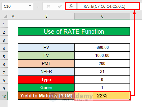
The RATE function does not work for some combinations. In these cases, the #NUM! error occurs. To solve this error simply add the Type and the Guess arguments in the RATE function. For Type, 0 or omitted is used for at the end of the period and 1 is used for at the beginning of the period. If RATE does not converge, try different values for the guess. RATE usually converges if the guess is between 0 and 1.
Using these two arguments, you can solve the #NUM! Error. Look at the below screenshot.
Please download the Excel file for your practice.
https://www.exceldemy.com/wp-content/uploads/2022/09/Calculate-Yield-to-Maturity.xlsx
Regards
Md. Abdur Rahim Rasel (Exceldemy Team)