Latest Posts From Abrar-ur-Rahman Niloy

What Are Major Gridlines? Major gridlines divide the chart axis into major units. Major gridlines are vertical or horizontal lines that represent the axis ...

Method 1 - Inserting Page Number in Excel Cell Step 1: Open VBA Window VBA has its own separate window. You must insert the code in this window, too. To ...

While collaborating with others on a worksheet, the updates are auto-saved. Changing in one section automatically changes the other. This goes for views too. ...
![[Fixed!] Excel File Too Large for No Reason (10 Possible Solutions)](https://www.exceldemy.com/wp-content/uploads/2022/07/excel-file-too-large-for-no-reason-3.png?v=1697110295)
Fix 1 - Check for Hidden Worksheets Increasing the Excel File Size For example, let’s take a look at a workbook with a hidden sheet. The sheet tabs at the ...

This tutorial will guide you on how to make Excel spreadsheets easier on the eyes and pleasing to work with. 12 Quick Tips to Make Excel Easier on the ...

The usual label printing process from Microsoft Excel involves mail merging spreadsheets with Microsoft Word. But some people prefer completing all the chores ...

Method 1 - Change 'Cell Errors As' Option Steps: Go to the Page Layout tab on your ribbon. Select Print Titles from the Page Setup group or the ...

Dragging is a quick and easy way to create a number sequence in Excel. But there are scenarios where you might want to create one without dragging the fill ...

Finding the slope of a linear trendline is relatively straightforward in Excel. You just have to find out the equation and declare the coefficient of x from ...

What Is a Gantt Chart? The Gantt chart was popularized by Henry Gantt. It is a type of bar chart that illustrates or tracks a project schedule. It ...

The following dataset will be used to create dynamic charts in Excel using data filters. Method 1 - Filtering the Dataset to Create Dynamic Charts ...
Example 1 - Plot a Stacked Bar Chart from an Excel Pivot Table This is the sample dataset. To Create a Pivot Table: Select the whole dataset ...
Method 1 - Using Context Menu Steps: Right-click on the column that is represented by the legend you are trying to change the color. The context menu ...
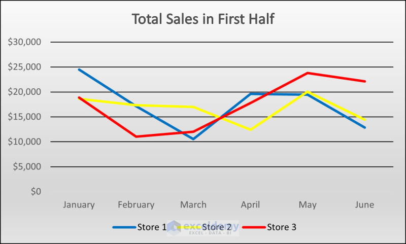
We will plot the types of graphs from the same dataset, which is below. The dataset includes sales of different stores in different months. All months are ...

We are going to convert each entry in the following dataset into a QR code in an Excel spreadsheet and scan them to find if they are working as intended. ...
- « Previous Page
- 1
- 2
- 3
- 4
- 5
- 6
- …
- 8
- Next Page »
See Our Reviews at


Hello Richard!
You need to replace 0s in the format type with 0.00s.
For example, instead of #,##0_) ;(#,##0) for center alignment, use #,##0.00_) ;(#,##0.00).
Regards
Niloy
Team Exceldemy
Hello Mahmoud,
Looks like there were several inconsistencies in your code. This is the modified version of your code:
Try out this one. It should work fine.
Hello again, Jessica! In the previous reply, I have mentioned exactly how you can do this. If you go through the second step, you will find the item number of your second Outlook mail (generally is 2. can also be 1 depending on how you had logged in to your accounts).
If it isn’t, take note of the number. Replace the 2 in .SendUsingAccount = mApp.Session.Accounts(2) with the number Excel shows. You will find this line in the With statement at the end.
In case if you are having trouble understanding any of the part, let us know about that.
Hello, Khurram Javed!
As of the latest version of Excel, the SUMIFS function doesn’t support partial matches with numbers directly. If your codes contain alphanumeric characters then the formula works perfectly. Because Excel doesn’t recognize them as “number” format.
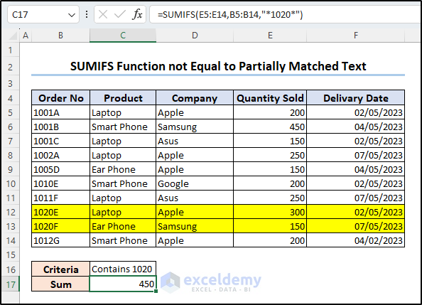
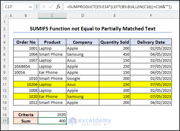
If the range B5:B14 contains numeric values only (i.e. 102054), the function will return a #VALUE! error saying wrong data type.
However, if you are only concerned with the result and not with the formula, there is a workaround for that.
Hi, Jessica!
Yes, it is possible. In short, Outlook assigns every email of yours to a number. You can call a specific mail using the Accounts.Item(x) method, x is the number assigned to the mail. Mention this account in the MailItem.SendUsingAccount property and the code will send the mail from that specific account. Keep in mind, the process works for Excel 2007 and later versions.
Here is the details of the process:
(This is to enable the Outlook library in your Excel workbook)
This code will give you the list containing your outlook mails and their numbers on your spreadsheet.
Hope this helped. If you still have inquiries, let us know.
Hi, Icide. M. O.
VLOOKUP or XLOOKUP is specifically for finding a value from a table/range. If you have the CGPA already calculated, you can use these functions to find it like this.
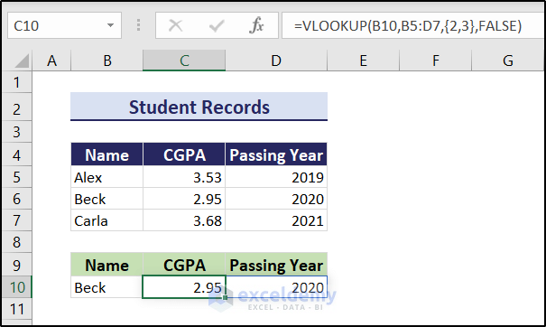
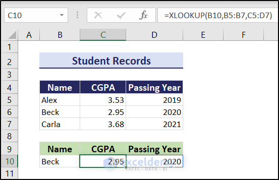
Similarly, you can use the XLOOKUP function too.
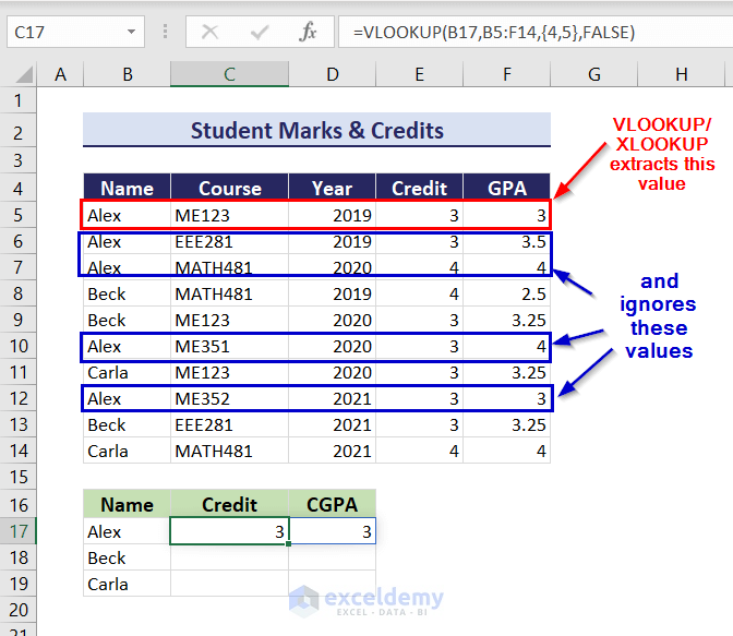
Assuming you don’t have the CGPAs already calculated, you want to do that from grades within Excel, you need all the grades for a certain person. If you have multiple values matching in a range, the VLOOKUP/XLOOKUP only returns the first match.
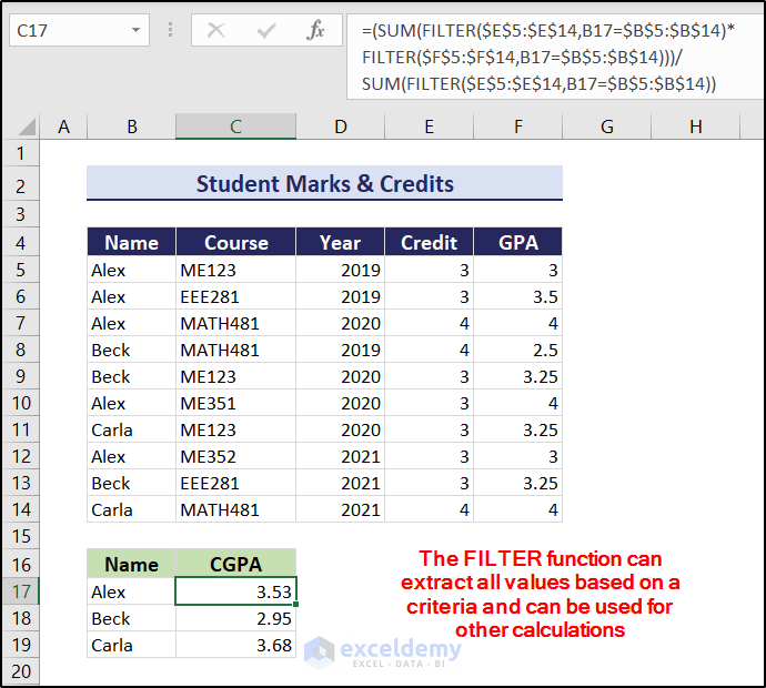
However, there are other workarounds for this. For example, the FILTER function can extract all the matching values. You can use them to your calculation’s advantage after that.
Here, I have used the Σfixi/Σfi formula to calculate the CGPA assuming it has a credit system. I have also used the absolute referencing as you have mentioned replicating the formula for a group of students. Hopefully, this answered your question.
If you are still struggling with your particular dataset, feel free to let me know. I will try to get back to you.
Regards
Niloy, Team Exceldemy
Hi Nawaf, thanks for the appreciation!
We focused more on the checklist side of the task tracker- whether or not the task is done or yet to be done (or not) was our main focus here. Also, we wanted to rearrange and prioritize our tasks based on a criteria. So we skipped the timestamps in this article. If that is your priority, you can easily do so too by adding an extra column and including it within the dataset too.
You can also add an assigned time and current time and compare them to find the status of the task in the main dataset. If you face any problem regarding the timestamps or want to do something particular with them, let us know. We are always here to assist.
Thanks again, there seems to be some cache from the recently opened office files in the location. Deleting them would certainly help.
Thank you for pointing this out. There are some cache files in the location and the article has been updated for later uses.
Hello Aniket!
As of now, we are only focusing on Microsoft Excel for Windows. But in case of other versions, there are some shortcut keys that do not work for iPad yet. It is constantly getting updated. If only some of the shortcuts aren’t working for you, then that may be the case. One solution would be to stay up to date with their updates.
Hi Elly,
For your data, plotting a stacked bar chart would not be possible. Excel needs a dataset of the following sort to plot a stacked bar chart.
1st Week 2nd Week 3rd Week 4th Week
1st Task 44 41 61 58
2nd Task 38 52 53 64
3rd Task 42 48 50 56
4th Task 37 59 44 46
Even in that case, creating a Gantt chart would not be appropriate, as one bar will start where the previous one ended. This will ultimately result in the same bar plot. But if you have a gap between each work period, you can put them in between these values and follow the steps of the article.
Hi, Patrick James O’Connell.
It is pretty “suite” you found it amazing. But unfortunately, there is no way to keep formats while joining strings together up until the latest version till date. Excel doesn’t even keep the formats of dates and times, so we have to go through these TEXT functions to keep that format.
Glad that it was helpful to you, Troy. Stay with us for more of these stuffs in the future.
Hi, sbellmore
This happens because of the .UsedRange method in the 13th line in the code.
Set Rng = Worksheets(Work_Sheets(i)).UsedRange
You can replace .UsedRange with .Range method to put one dataset or a particular portion of the dataset (eg without headers). For example, with our dataset, you can use the following.
Set Rng = Worksheets(Work_Sheets(i)).Range(“B4:C7”)
or,
Set Rng = Worksheets(Work_Sheets(i)).Range(“B4”).End(xlDown).End(xlToRight)
The downside of using such lines of code is, if you have any dataset without headers, it may ignore the part or whole dataset in some cases. As some of your sheets may not contain a dataset starting from cell B7. For automation, unfortunately, using .UsedRange is the most efficient method.
Sorry for the inconvenience. It has been fixed.
Hi Scott. Unfortunately, no, there isn’t. If you pass your password to a client and if he chooses to share it with anyone else they will be able to access the file too. It’s a limitation like any other login service.
Hi Kheiy. Yes, there is an easy way to do that. Go to the Mailings tab on the word file and select Finish & Merge. Then select Print Documents from the drop-down. After that, you can find the option to print all pages or a particular range if you want.
Hi Raj,
Do you want to put all the row values in a single cell? You can try out the following formula to concatenate them. But it will be converted into a string.
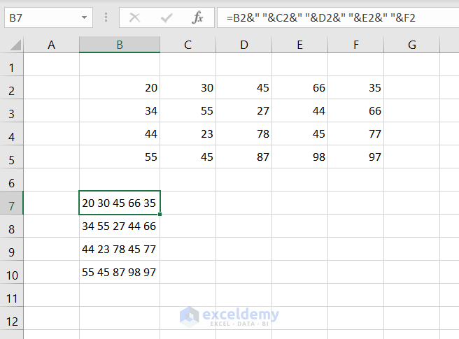
If you want to know something else entirely, kindly elaborate on your problem. We will try to help the best we can.
Glad it had been helpful for you.
Hi Gerald,
You can create certain data tables consisting of probability. Provide us with more details, we will be able to help with the detailed procedures.
Click on “Enable Editing” in the message that appears above the formula box.
Hi Brian,
The article mainly focuses on the mortgage calculator between two parties. For an escrow, if there are no conditions involved, it will look almost the same.
We are glad that this helped.
Hi Romesh.
IRR is not the sole measure of comparing profitability. It is just one of the many parameters you can use to compare two paths of investment.
Hi Colvis.
We are very sorry for not reaching out to you promptly. But the annual IRR is calculated by multiplying the monthly IRR by 12. In that case, we get an annual IRR value of 6.504%. The value of IRR from the IRR formula and the XIRR formula should not be the same for irregular cash flows. And these values reflect that.
Hi Temitope,
Our website currently focuses on providing articles and solutions for Microsoft Excel only. If you have the same problem in Excel, please provide us with a little bit more information. We will try to assist you as much as possible.
Hi SteelWolf,
I am not sure what you meant exactly by that. But assuming you want to put in a date in cells F6, H6, J6, L6, N6, P6, and R6 that match with cell J1, you can use formulas in those cells with reference to cell J1. For example, let’s assume you want the previous date, exact date, and the following date of cell J1 in cells F6, H6, and J6.
You can write =J6 in cell H6. Write =EDATE(J6,-1) in cell F6 and =EDATE(J6,1) in J6.
You can modify/ use different formula according to your needs in this way.
But if you want you use the “autofill” in those scattering cells, it is not possible yet as of the latest version of Excel.
Hope that helps. If you meant something else entirely, please let us know.
Hi Cris,
I am so sorry for your situation. But we haven’t worked with the iPhone platform yet. So our solutions are only limited to windows for now.
Hi Elona,
I am not sure I understand your problem quite clearly. But if you are having problems importing data from different sheets, then put the sheet name before the range in single quotes followed by an exclamation sign.
For example, you should add ‘Sheet 2’! before the range G3:G123 or any other range while using them as the source to use formulas in the first sheet.
Hi Debbie,
Yes, you can use multiple criteria for the MATCH function. Try it like this:
MATCH(1,(first criteria)*(second criteria)*(third criteria),0)
in place of the match function used for a single criterion.
hi Willy,
Make sure the file names are correctly spelled in the line. Check if both the source file and target file name are correct as well as if the directory of the workbook file is correct too.
If the problem still persists, please provide us with a bit of more information, like what is the error message or perhaps a screenshot.
Hi Eric, the COUNTA function counts all the cells including empty strings. It ignores a cell only if there was no value entered or you have deleted it completely (pressing delete or erasing the entire cell value).
But if you use the COUNTBLANK function to count the same range, you will find that the empty strings will indeed are being counted as blank values.
Hi Jeff, so sorry for your unfortunate situation. But the formulas are structured in such ways that it returns empty strings if only certain criteria are met. It won’t result in entire rows or columns being empty.
Hi Akhil,
Unfortunately, there are no direct ways or simple formulas to do that. One way to work around this is to remove the columns as the entirety of them is empty. And then try transposing. Or you can try out VBA to remove the empty columns/rows then try using transpose commands.
Hi Esayas,
You can count that if you mix the formulas with the COUNTIF function. You have to be a bit creative while using it in VBAs. For example, take the first method. You can use =TEXTJOIN(“, “,TRUE,IF(C14=B5:B12,C5:C12&”:”&COUNTIF(C5:C12,IF(B5:B12=C14,C5:C12)),””)) formula instead of the given one to find the count of each one in the dataset along with the models.
Hi Vikas,
Seems like your first problem meets the criteria for this article . In the ending date cell, try using the TODAY function, and at the starting date put in the formula =EDATE(TODAY(),-5).
As for your second criteria, use the formula =EDATE(TODAY(),-5) of this article’s current cell value instead of today’s date and that should do the trick.
Hope that helped. If you are still facing issues, or you wanted a different result let us know.
Hi Jose,
You can choose any of the three methods given above to remove the “↑” sign. All of them work for any non-numeric character, including the one you are asking.
Hope that helped. If you are still facing problems, let us know.
Hello, SAF. I am glad it was helpful to you. As for your problem, you don’t need to reupload every time you enter new patient names in Excel.
You can select “Edit Recipient List”> select the file name in the “Data Source” section and hit refresh. It will automatically update the recipients’ list up to the latest entry.