Latest Posts From Mohammad Shah Miran

Method 1 - Create a 2-D Stacked Bar Chart with Negative Values Step 1: Insert Stacked Bar Chart Select range C5:F10, go to the Insert tab >> Charts ...

Consider the following dataset with some order information. We'll use SUMIF with AND to comb through the data. Example 1 - Application of SUMIF and ...

Basics of Variance and Standard Deviation Variance examines how distinct numerical values relate to one another within a data collection. It treats all values ...

When you work with a large set of data, your data may disperse in several sheets of your Excel file. A dynamic drop-down list can help you to accumulate that ...

For a number of tasks and uses, including financial analysis to sales forecast, Excel will continue to be a crucial tool for enterprises. For instance, you can ...
Step 1 - Prepare the Dataset Dataset Selection: Assume we have a dataset named “Project Timeline of ABC Multipurpose Bridge.” However, feel free to ...

“Product Price of ABC Beverage Limited” is the sample dataset. Example 1 - Creating a Decision Tree for 4 Events Step 1: Construct Essential Shapes ...

Networking equipment such as switches, routers, wireless, etc. is well-known in the technology industry. To promote the product, companies may often require to ...
Method 1 - Using Parametric Estimation Steps: Enter the following formula in cell G5. =C5/(D5*E5*F5) Drag the Fill Handle tool to get the ...

Below is our dataset called “Running Project of DPR Construction”. Step 1: Open a Dataset from OneDrive Using Desktop App Go to your dataset ...

The VBA Union method helps to put several ranges into one single range. You can also find and sort a wide range of data into one single range based on specific ...
Method 1 - Employ VBA Code in Module Press Alt + F11 to open your Microsoft Visual Basic. Press Insert > Module to open a blank module. ...
Formula to Calculate Kurtosis Despite having a biased estimation if you do not have the full-scale data of a given phenomenon, we will calculate the ...
![[Solved!] Excel Spin Button Not Working (2 Reasons with Solutions)](https://www.exceldemy.com/wp-content/uploads/2022/12/Sprint-Button-Fixation-2.2.png?v=1697451730)
While using the spin button in Excel, users can choose a numerical value from a predetermined range. These buttons appear as scroll bars without the scroll and ...

Complex numbers are expressed as a+ib, where “a” is a real part of the complex number and “b” is an imaginary part of the complex number. For instance, the ...
See Our Reviews at


Yes AS, you are correct. The article has been revised. Thanks for noticing this and letting us know.
Regards
Mohammad Shah Miran
Team ExcelDemy
Thank you PAULO GIOLO, for your query. Yes, I have just checked and found there is no issue to
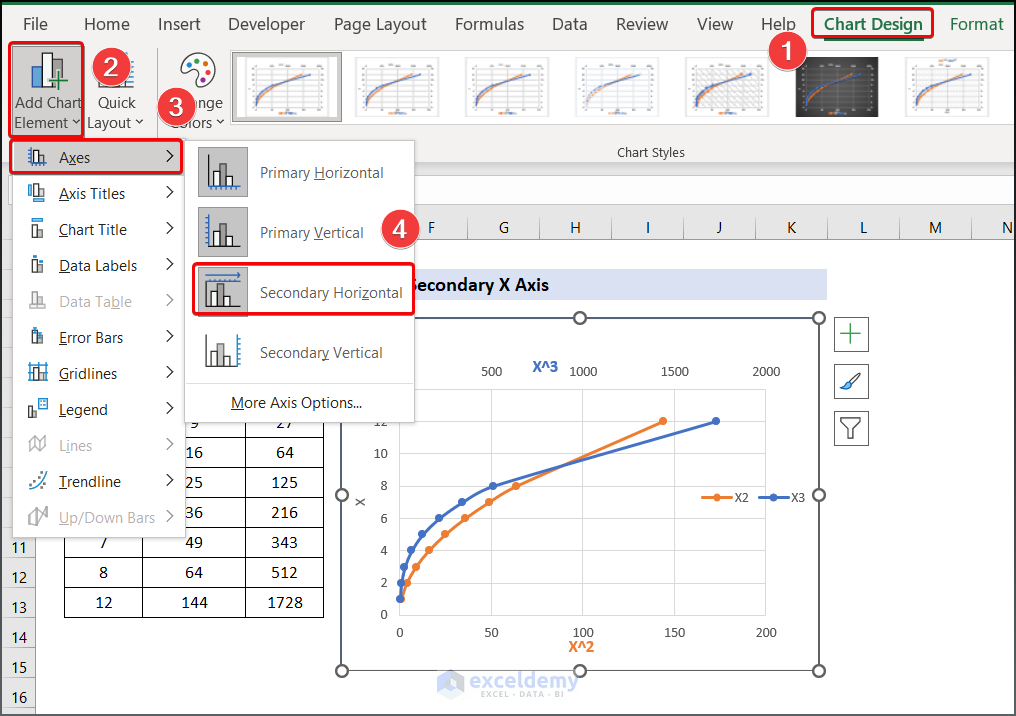
enable the secondary axis which is embedded in the PowerPoint slide. If you are missing plus sign in your chart, there is an alternate way that has been illustrated by the image below.
However, if there is no secondary horizontal axis option in the Chart Elements, then follow this part of the article. https://www.exceldemy.com/add-secondary-x-axis-in-excel/#Excel_Not_Showing_Secondary_Horizontal_Axis_Option
Hope this will work for you. If you have further queries, feel free to ask.
Regards
Mohammad Shah Miran
Team ExcelDemy
Thanks, MIKE M for your question. The problem you are stating indicates that the Solver could not find a solution that satisfied the optimization constraints you specified. This can happen for several reasons, including Incorrect input data, Incorrect model specification, Insufficient or incorrect constraints, Numerical instability, etc. Try to rectify those issues or if you need a more specific solution to your problem, it would be convenient if you provide your dataset. Thanks for being with ExcelDemy.
Regards
Mohammad Shah Miran
Team ExcelDemy
Thank you SHASHI, for your query. I think this article might help to solve your problem.
https://www.exceldemy.com/count-colored-cells-in-excel/#3_Utilizing_GETCELL_4_Macro_and_COUNTIFS_Functions
You can try to use this method for Conditional Formatted cells also. Further, if you have any confusion or query related to it, please let us know.
Thank you, Jeb, for your query. You can take the API as a String value to your VBA code. Thus you don’t need to put the API value in your Excel sheet. So the existing code given in the workbook here can be modified as follows:
Here we have changed the first two line of the given code. The previous code was as like:
But we have removed the third argument which represents the API value. Alternately, We declare the variable outside and put the API as a string value.
Now here comes to your second question. You have to create a customized Add-in to store your VBA code and therefore allow you to execute the code in any workbook. Hope you get your answer. However, if you have any further query, please let me know.
Thank you, Hossam for your query. I am not sure whether you alter AVERAGEIF with AVERAGEIFS. If so, there should be a difference between them as AVERAGEIF deals with single criterion whereas AVERAGEIFS deals with multiple criteria. However, you can use the AVERAGEIFS function for a single criterion by specifying only one criterion range and one criterion. For example, you have a range of cells A1:A10 that contains numbers and you want to calculate the average of the cells that are greater than or equal to 5. For accomplish your task, you can use the AVERAGEIFS function like this:
=AVERAGEIFS(A1:A10, A1:A10, ">=5")Further if you have any query, please let me know. Thank you.
Thank you VIRGIAL for your query. Yes, you can use the COUNTIF function to count the number of items that have broken the Conditional Formatting threshold value. For doing this, write down the following formula in your desired cell. (eg. D11)
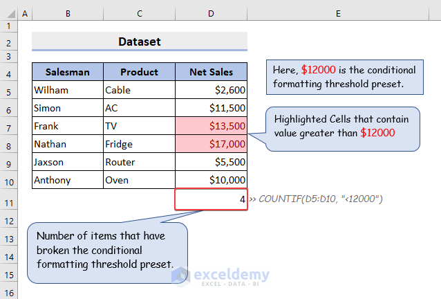
=COUNTIF(D5:D10, "<12000")Here, D5:D10 is the data range for which you want to set your condition and 12000 is the Conditional Formatting threshold value.
Additionally, the following image can be useful to comprehend the task.
Thank you, Greg Erkins, for believing in ExcelDemy.
Use the following Macro Code to get your desired output.
To aim the output, I have written the function name UrlConstructor and called friendly name and range of country code as an argument, like the picture given below.
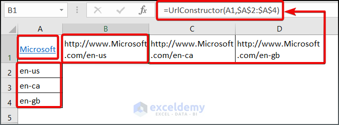
Download the Excel file for your better assistance (URL Construction from Friendly Name.xlsm). Also, let us know if you wish to learn more or have any concerns relevant to it. Good luck!
Thank you for getting in touch with us. Based on your comment, what i understand is that you are interested in creating a schedule to track your maintenance work. I have provided an Excel file (Machine Maintenance Schedule) that outlines the different types of work you will need to perform. However, I would like to confirm whether your MNT1 and MNT2 etc. tasks are repetitive, or if they only need to be completed once every 15 days.
If you would like to automate this process, you can incorporate a nested for loop to generate the desired output. Additionally, you can develop a sub-function to prevent repetitive values from being generated.
Further, if you have any questions or concerns about this matter, leave your query here. We are here to help and are at your disposal.
Hello Imran,
Thanks for the query. What I understand from your comment is that you want to incorporate a VBA code for the formula instead of going to the formula editor. Here are my two cents which might help you in this regard. Look at the dataset attached below.
After pressing the ALT+F11 short key to open your VBA window, paste the following code in the Module box.
Save & Close your VBA window. Then, press F8 to open the Macro dialog box and click on Options.
Create a shortcut key to make the process fast, Crtl+W for instance.
Now see the output as given below.
Hope you have got your answer. Good Luck!
Regards
Miran
Excel & VBA Content Developer