Latest Posts From Zehad Rian Jim
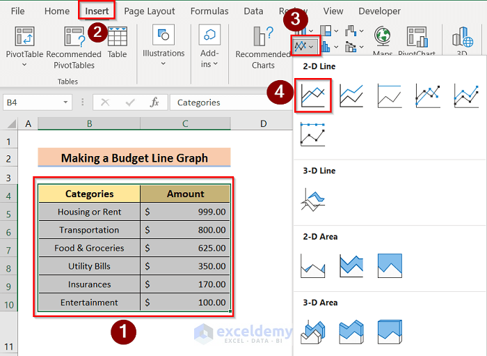
This tutorial will demonstrate how to make a budget line graph in Excel. A line graph is a statistical graphic to highlights the numerical proportions of a ...

This tutorial will demonstrate how to create Bubble Chart with 2 Variables in Excel. A bubble chart is very useful in interpreting charts. You can use it to ...

This tutorial will demonstrate how to calculate the issue price of a bond in Excel. In Microsoft Excel, you can easily calculate the present value of a bond. ...

This tutorial will demonstrate the steps to show coordinates in an excel graph. Undoubtedly, graphs are very useful for easily representing any collected data. ...

Step 1: Arranging Dataset Put the Name in column B, the Starting Time in column C, and the Actual Time in column D. We will use this dataset throughout. ...

The AVERAGEIF function returns the average of the cells of an array that satisfy one or more given criteria, which can be from the same array or a different ...

Overview of INDEX Function Description: It returns a value or reference of the cell at the intersection of a particular row and column, in a given ...
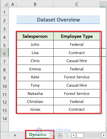
The sample dataset is an overview. Method 1 - Using in VLOOKUP Function on Each Sheet Individually Steps: Create a dataset as shown below. ...

This tutorial will demonstrate how to display the references dialog box in Excel. When you are dealing with lots of VBA codes in a different worksheet in a ...
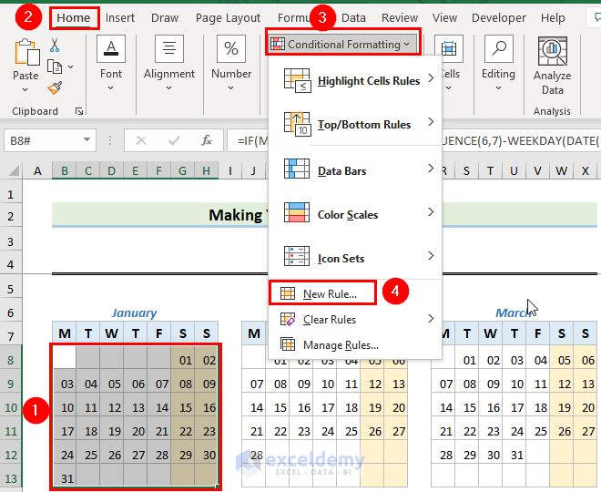
This tutorial will demonstrate how to make a calendar in Excel without a template. In our day-to-day life, we all use a deadline for certain work or projects, ...

This tutorial will demonstrate how to insert a radio button input box using VBA in Excel. Radio buttons are mainly used as options in cases where different ...

This tutorial will demonstrate how to make a balance sheet format in Excel for an individual. A balance sheet is important when it comes to a proprietorship ...
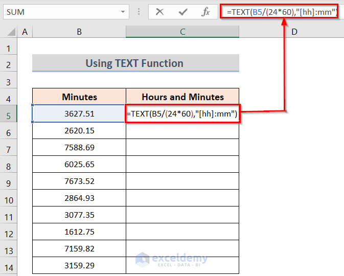
Method 1 - Use Excel TEXT Function to Convert Minutes to Hours and Minutes Steps: In the C5 cell insert the following formula. ...
We’ll use a sample dataset, with Input in column B and the Timestamp in column C. We'll input the timestamp in column C whenever we modify the respective cell ...

We'll use a simple dataset to showcase how you can select values in a column to the end of data. Method 1 - Using a Keyboard Shortcut to Select ...
See Our Reviews at


Hello DESTINY,
First, thanks for your curious question. It was amusing to solve the problem. Let me guide you to fulfill your query.
Step 1. Assume you have a Dataset where you have the Names of the employees in one column and the types of the employees in another.
Step 2. Then insert the following code in the VBA window.
Sub Copy_Rows_3()
Dim r1 As Range, Row_Last As Long, sht As Worksheet
Dim Row_Last1 As Long
Dim src As Worksheet
‘Change this to the sheet with the data on
Set src = Sheets(“Dynamic”)
Row_Last = src.Cells(Cells.Rows.Count, “C”).End(xlUp).Row
For Each r1 In src.Range(“C5:C13” & Row_Last)
On Error Resume Next
Set sht = Sheets(CStr(r1.Value))
On Error GoTo 0
If sht Is Nothing Then
Worksheets.Add(After:=Worksheets(Worksheets.Count)).Name = CStr(r1.Value)
‘Sheets(CStr(r.Value)).Cells(1, 1) = “Total”
Row_Last1 = Sheets(CStr(r1.Value)).Cells(Cells.Rows.Count, “B”).End(xlUp).Row
src.Rows(r1.Row).Copy Sheets(CStr(r1.Value)).Cells(Row_Last1 + 1, 1)
Sheets(CStr(r1.Value)).Cells(1, 2) = WorksheetFunction.Sum(Sheets(CStr(r1.Value)).Columns(3))
Set sht = Nothing
Else
‘Sheets(CStr(r.Value)).Cells(1, 1) = “Total”
Row_Last1 = Sheets(CStr(r1.Value)).Cells(Cells.Rows.Count, “B”).End(xlUp).Row
src.Rows(r1.Row).Copy Sheets(CStr(r1.Value)).Cells(Row_Last1 + 1, 1)
Sheets(CStr(r1.Value)).Cells(1, 2) = WorksheetFunction.Sum(Sheets(CStr(r1.Value)).Columns(3))
Set sht = Nothing
End If
Next r1
End Sub
N.B. if you are following our article, use the VBA code under the method “Copy Rows in Excel to Another Sheet Dynamically” and change the marked portions.
Step 3. After pressing Run, you will get the result in individual desired cells.
Thanks
At first, Create a dataset having Age in Column B, Fixed Amount in Column C and Principle At the Start of the period in Column D.
Then, insert the following formula in cell D5 and use the Fill Handle option to apply it to all cells of column D.
=B5*C5
Finally, insert the following formula in cell E6 and use the Fill Handle option to apply it to all cells of column E to get the desired result.
=E5*(1+0.02)+D6
The excel file is added here according to your wish.
Compound Interest Statement.xlsx
Thanks and happy helping.
Hello CALEY FORBES,
Thanks for the amazing question. Let me guide you in solving this problem.
First, I want to solve your first query. I think to solve your problem it is better to use our first method ‘Automatically Copy Rows in Excel to Another Sheet Using Filters’ method than using VBA code. The reason behind this is I think the first method will do your desired work without hesitation.
For the second query, you have to insert the following formula in the VBA windows.
Sub Cut_Range_To_Clipboard()
Range(“B4:B10”).Cut ‘This will cut the source range and copy the Range “B4:B10” data into Clipboard
‘Now you can select any range and paste there
Range(“J2”).Select
ActiveSheet.Paste
End Sub
Note: in the Range section you can change the desired option to paste accordingly.
I hope, your problem will be solved in this way. You can share more problems in an email at [email protected]
Happy Excelling!!!
Thanks Deep for your excellent and thoughtful question. Let me guide you to fulfill your query.
We can easily extract multiple texts in cells by using different methods of this article but with slight changes.
Suppose you have a dataset where the texts are separated only with hyphens. In this scenario, you should follow the first method in our article. The steps are:
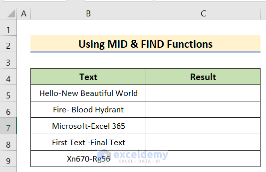
First, arrange the dataset where texts are separated with hyphens.
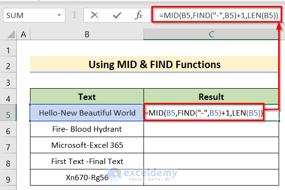
Second, insert the following formula.
=MID(B5,FIND("-",B5)+1,LEN(B5))Third, after pressing Enter button, you will get the result for this cell.
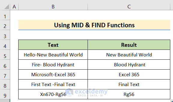
Last, use the Fill Handle to apply it to all Cells.
But in case, you have emails separated with @ or any other texts separated with special characters then you can use RIGHT, SEARCH & SUBSTITUTE Functions or LEFT, FIND & SUBSTITUTE Functions or RIGHT, REPT & SUBSTITUTE Functions from our article.
Any of these methods will do the work for you. Let me guide you in detail with the steps.
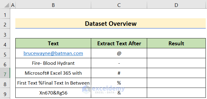
Firstly, you must arrange a dataset where multiple texts are separated with special characters.
Next, use any of the following formulas in the D5 cell(described in our article)
=RIGHT(B5,LEN(B5)-SEARCH("#",SUBSTITUTE(B5,C5,"#",LEN(B5)-LEN(SUBSTITUTE(B5,C5,"")))))or
=SUBSTITUTE(B5,LEFT(B5,FIND(C5,B5)),"")or,
=TRIM(RIGHT(SUBSTITUTE(B5,C5,REPT(" ",LEN(B5))),LEN(B5)))(Note: Please take a glimpse at our main article to understand the insertion of the formula)
Afterward, after pressing Enter button, you will get the result for this cell. You will get the same result for any of the formulas so you can choose any of them.
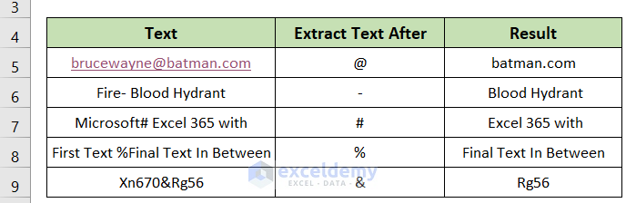
Last, use the Fill Handle to apply it to all Cells.
Thanks, RICARDO SERRÃO for your two amazing queries. Let me help you out in solving your problems.
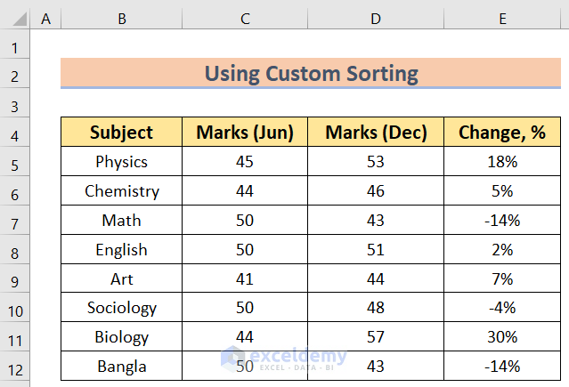
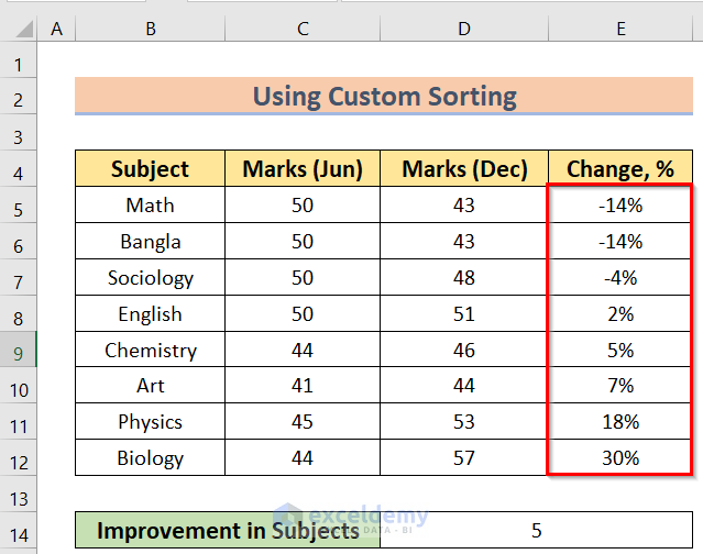
First, we are going to discuss your first question. The problem you faced is about custom sorting.
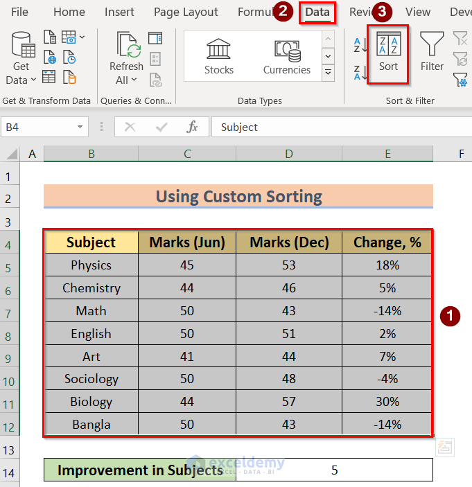
At the very beginning, we arranged a dataset of change in percentage.
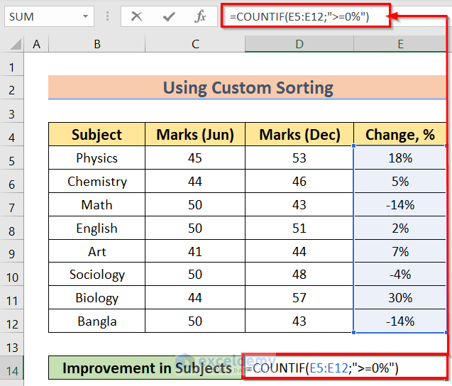
Then, as you wished we have used the COUNTIF function in this dataset.
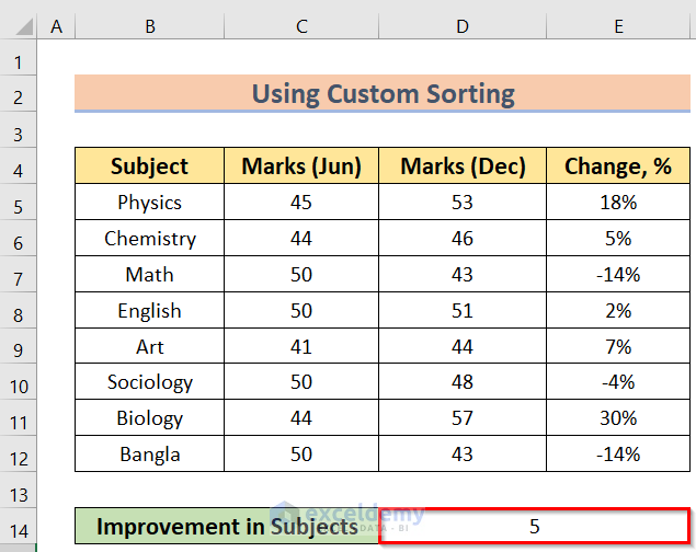
As a result, we have found the values.
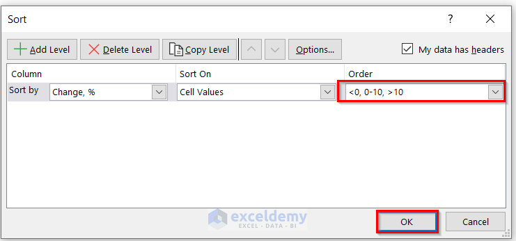
Now, select Dataset> go to Data>Sort options.
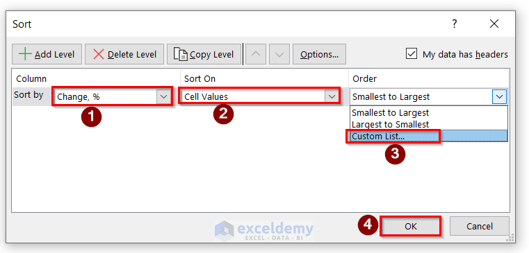
After that, in the Sort window, select Change% in Sort By option, Cell Values in Sort On option, and Custom List in the Order option. Press OK to execute it.
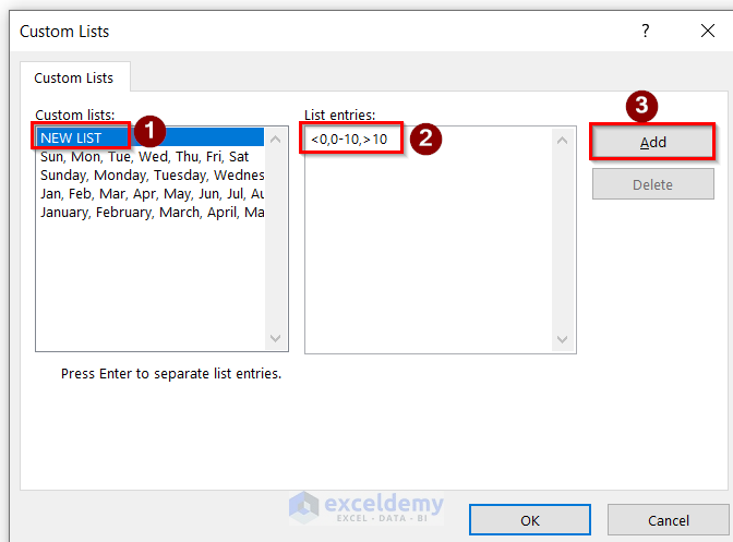
Furthermore, click on the NEW LIST option and write the condition manually in the List Entries area and press Add option.
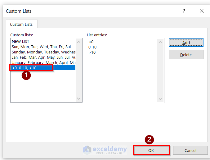
Because of that, you will get the desired condition in the Custom Lists section and press OK.
Afterward, if you can see the desired condition in the Order box then press OK.
Lastly, you will get the result accordingly. As in the condition, you have entered less than zero at first then zero to ten and at last greater than zero that’s why in the Excel section you will get the same order accordingly.
So, that’s the solution to your first query. Now, Let’s go through your second problem.
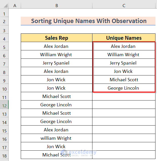
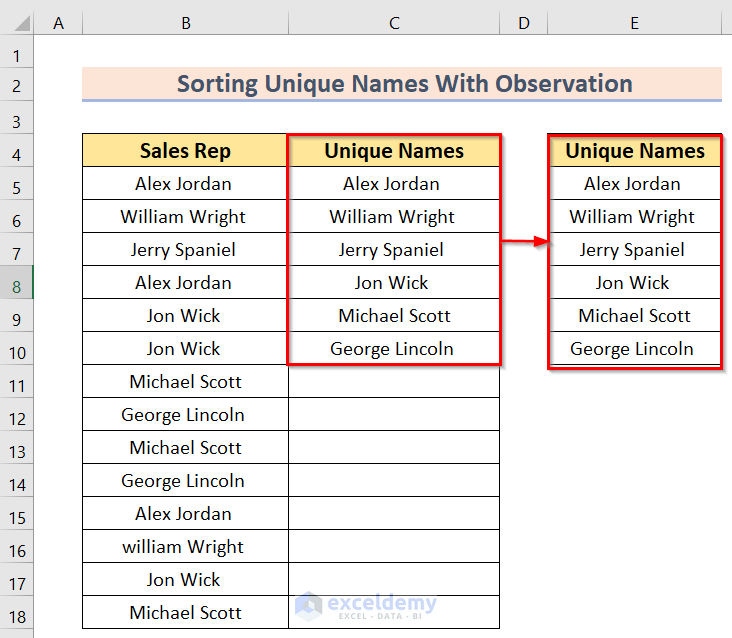
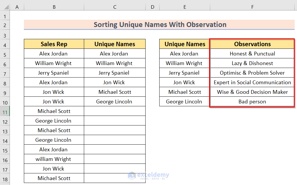
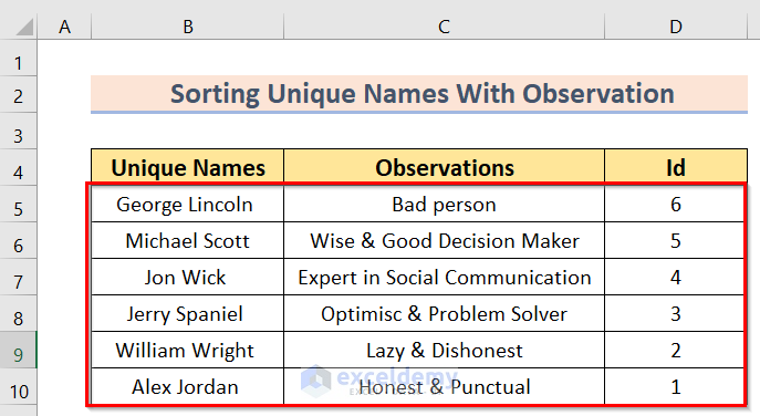
First, by reading your example, at first by using a formula, we created a Uniques Names list.
Second, you have to write down the same unique names list in another column. The behind this is, in the array, you can’t use sorting.
Third, then enter the Observations you made next to the new column.
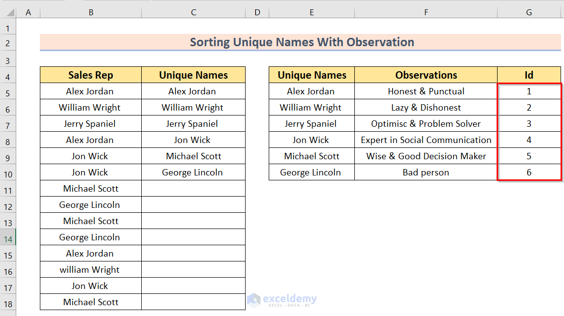
Forth, as we want to sort, so we mark each name with a unique Id number in a new column.
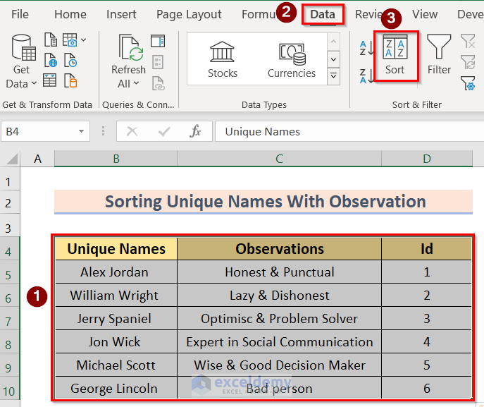
Fifth, go to select the table>Data>Sort options.
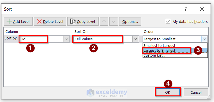
Sixth, select the Id option in the Sort by option, and Cell Values in the Sort On option, click on the Largest to Smallest option in the Order section, and press OK.
Finally, you will get the desired result.
So, this is the solution to your second query.
Therefore, our journey comes to an end. The problems were very fun to solve and I really feel amazed by helping you. Thank you once again. Best of luck.
Thanks, RON for your amazing question. Let me help you out in solving your problem. Please follow the below steps with us.
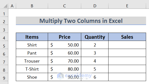
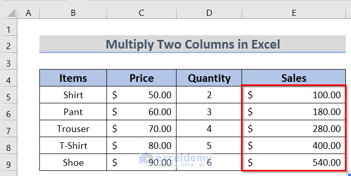
First, we arranged a dataset and add an extra column(in this case Sales) in the same table as the below image.
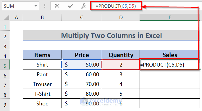
Then, insert the following formula in cell E5.
=PRODUCT(C5,D5)
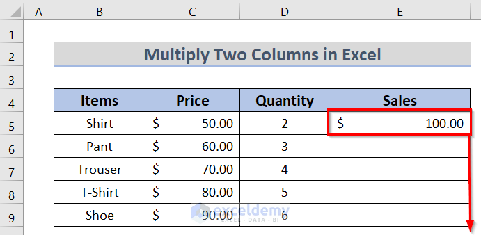
After that, if you press the Enter button, then you will get the result for that cell, and afterward, use the Fill Handle option to apply the formula to all cells.
Finally, you will get the desired result.
So, I have tried to solve the problem to multiply the cells in the same table. If you face any other confusion, then we request you to provide the Excel file and give us the opportunity to help you out. All the best.