Advanced Conditional Formatting Techniques in Excel

Image by Editor
 

Conditional Formatting is one of Excel’s most powerful features. While basic formatting can highlight cells based on simple rules (e.g., greater than or less than a value), advanced conditional formatting allows users to visualize data patterns, highlight important information, and create dynamic dashboards.

In this tutorial, we will show advanced techniques of conditional formatting and how to apply them in Excel.

1. Formula-Based Conditional Formatting

This technique allows you to apply formatting to a range of cells using a custom formula, offering maximum flexibility.

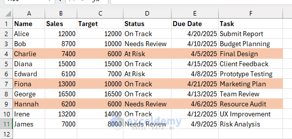
Let’s highlight entire rows where “Sales” are greater than the “Target”.

• Select the range you want to format (e.g., A2:F11 – entire data rows).
• Go to the Home tab >> select Conditional Formatting >> select New Rule.

• Choose “Use a formula to determine which cells to format”.
• Enter the following formula (assuming “Sales” is in column B and “Target” in column C):

=$B2>$C2

• Click Format >> choose a desired Fill color >> click OK.
• Click OK.

Explanation:

• This formula checks each row. If the value in column C is greater than column B, the row is formatted.
• The dollar sign ($C2) locks the column but not the row, so the formula applies correctly to all selected rows.

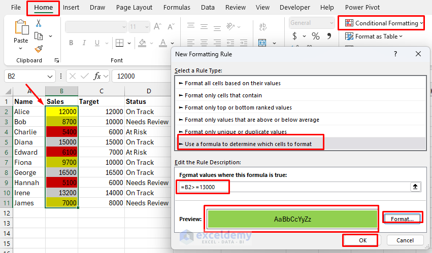
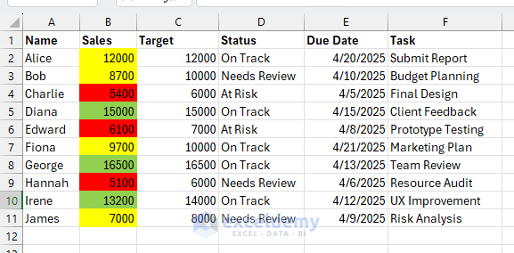
2. Apply Multiple Conditional Rules (Multi-tier Formatting)

You can apply different colors or formats based on multiple conditions.

Color-code performance:

• Red for low (<7000),
• Yellow for medium (7000–13000),
• Green for high (≥13000).

Steps:

• Select the data range (e.g., B2:B11).
• Go to Home tab >> select Conditional Formatting >> select New Rule.
• Use three different formula rules:
  • Low:

=B2<7000

• Apply a red fill.

• Medium:

=AND(B2>=7000, B2<13000)

• Apply a yellow fill.

• High:

=B2>=13000

• Apply a green fill.

Explanation:

Each condition is evaluated separately, and formatting is applied accordingly. You can prioritize rules if they overlap by using the Manage Rules option.

3. Customize Icon Sets, Data Bars, and Color Scales

These tools add visual cues directly inside cells, ideal for dashboards and comparative analysis. Visualize sales using data bars.

Data Bars:

• Select your range (e.g., B2:B11).
• Go to the Home tab >> select Conditional Formatting >> from Data Bars >> choose a style.

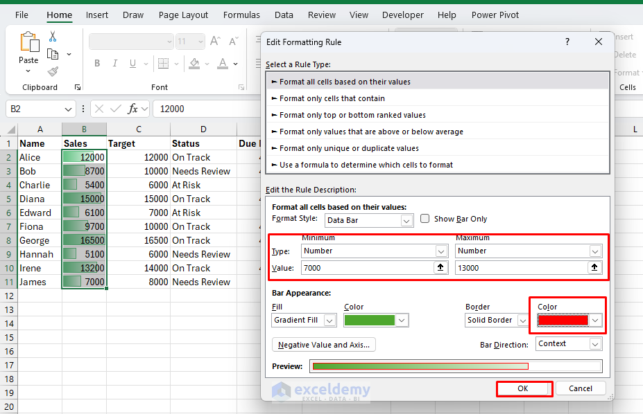
• If you want, you can customize the Data Bars.
• Go to Manage Rules >> select Edit Rule.

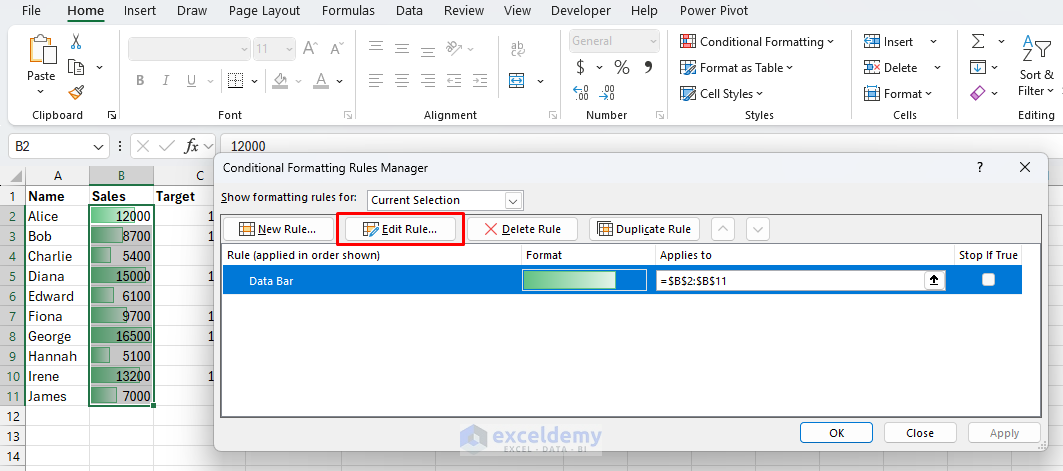
• Set Minimum and Maximum to Number for more control (instead of Percent).

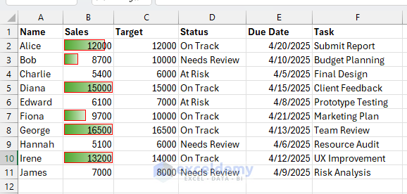
Output:

Color Scales:

• Select a range.
• Go to the Home tab >> from Conditional Formatting >> from Color Scales >> choose a set.
• Apply a 2-color or 3-color scale.

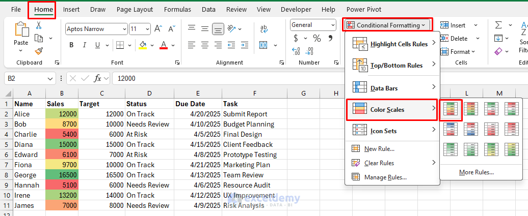
• You can adjust thresholds manually for fixed boundaries (e.g., min = 7000, max = 13000).

Icon Sets:

• Select your range (e.g., B2:B11).
• Go to the Home tab >> from Conditional Formatting >> from Icon Sets >> choose a set.

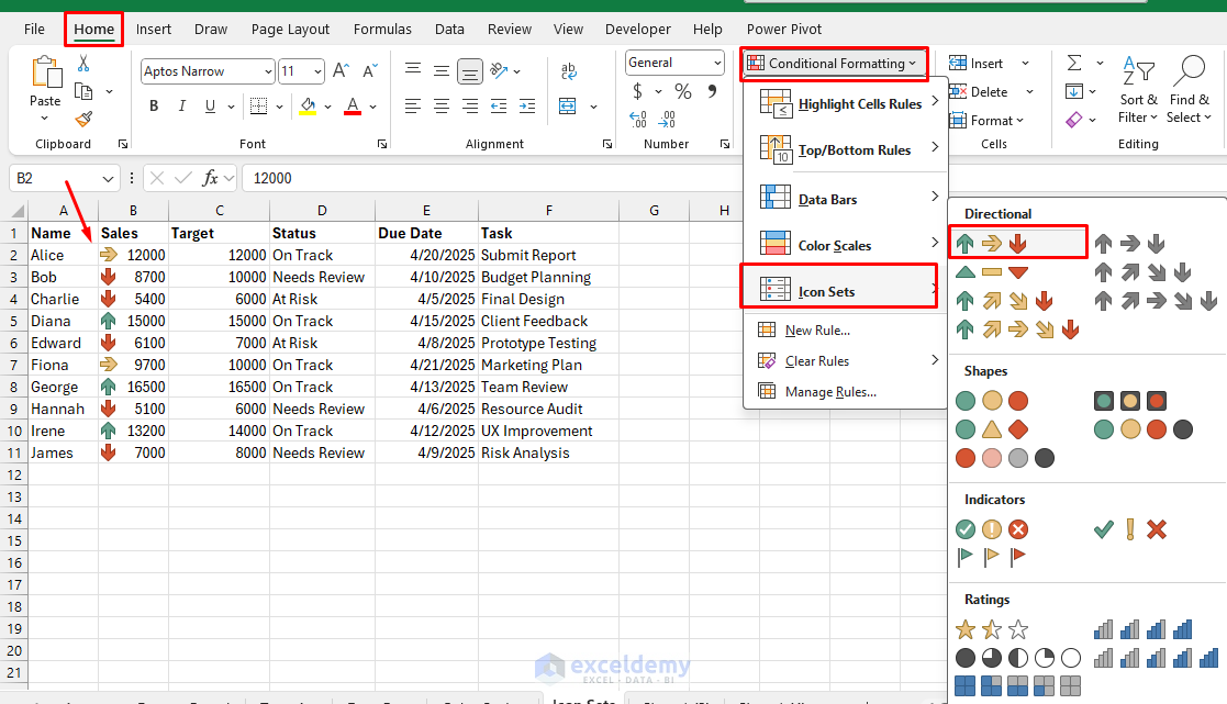
• You can Edit Rule, change the type from “Percent” to “Number”, and set custom thresholds like:

Note: You can use formulas to hide icons or combine them with other rules. You can use the Show Bar Only option to create a clean visualization without the underlying numbers.

4. Highlight Duplicate and Unique Values with Custom Logic

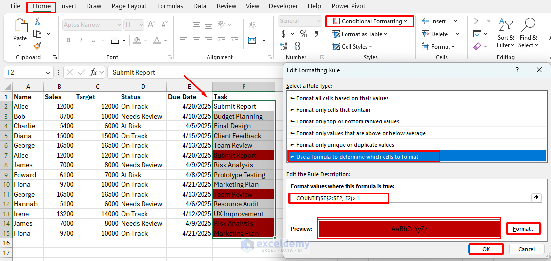
Built-in duplicate highlighting exists, but formula-based rules give more control. Highlight only second or later occurrences of a duplicate value in a column.

Highlight first occurrence only:

• Select your range (e.g., F2:F11).
• Use the formula:

=COUNTIF($F$2:$F2, F2)>1

• Format the result with dark red color.

Highlight duplicates across multiple columns:

• Select your range.
• Use the formula:

=COUNTIFS($A$2:$A2,A2,$B$2:$B2,B2)>1

• Format the result with red color.

Explanation:

• This formula counts how many times the value in the current row has occurred up to that row.
• If the count is greater than 1, it means it’s a duplicate occurrence.

5. Date-Based Conditional Formatting

You can highlight dates based on various conditions.

Highlight tasks due in the next 7 days:

• Select cell range (e.g., E2:E11).
• Use the following formula.

=AND($E2>=TODAY(), $E2<=TODAY()+7)

• Format the result with yellow color.

Highlight overdue tasks:

• Select cell range (e.g., E2:E11).
• Use the following formula.

=$E2<TODAY()

• Format the result with red color.

Explanation:

• The TODAY() function dynamically checks the current date.

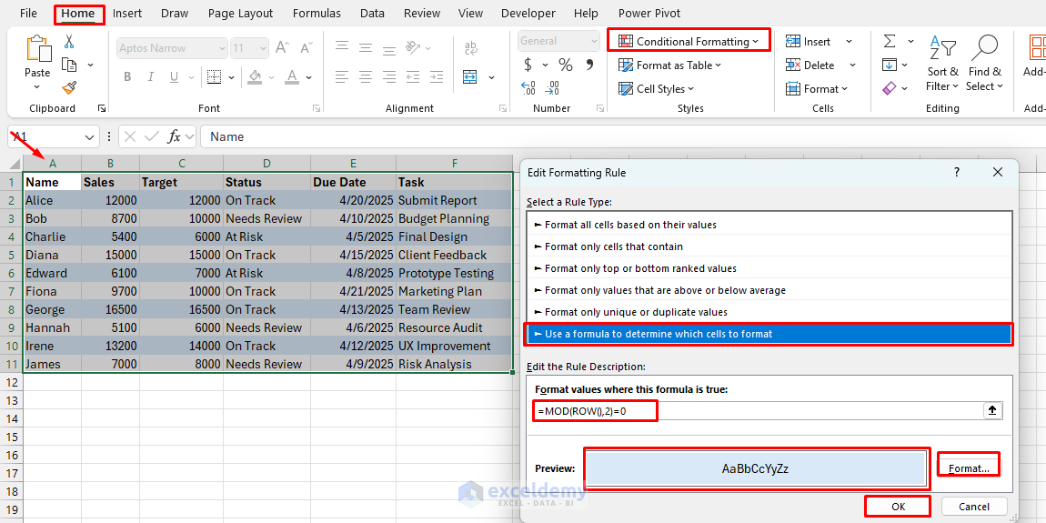
6. Create Alternating Row Colors Without Banding

You can customize alternating row colors using formulas.

For every two rows:

• Select cell range.
• Use the following formula.

=MOD(ROW(),2)=0

• Format the cell with a light blue color.

For every three rows:

• Select cell range.
• Use the following formula.

=MOD(ROW(),3)=0

• Format the result in gray color.

7. Interactive Formatting Using Dropdowns (Data Validation + Formatting)

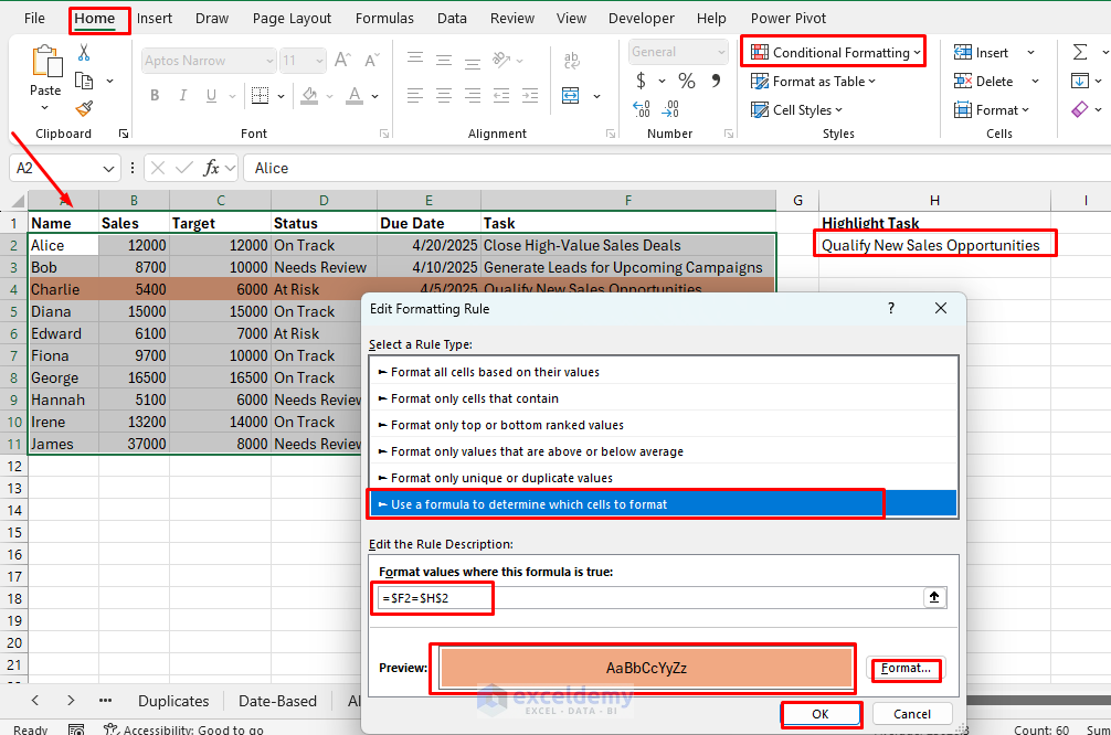
Make your formatting interactive based on a user-selected value. Highlight rows matching a category selected from a dropdown.

Steps:

• Create a dropdown in H2 with tasks from F2:F11.
• Select the entire row (e.g., A2:F11).
• Use this formula to highlight:

=$F2=$H$2

• Format the result with peach color.
• It dynamically highlights the row matching the selected task.

8. Use Named Ranges for Readability and Reuse

Named ranges improve formula clarity and reduce errors. Highlight the max value in a named range, e.g., SalesRange.

• Go to the Formulas tab >> select Name Manager >> select New.
• Name it SalesRange with reference:

='Named Range'!$B$2:$B$11

• Apply conditional formatting with a formula.

=B2=MAX(SalesRange)

• Format the result with green color.

9. Highlight Errors or Blank Cells

Helps in cleaning and validating data.

Highlight error cells:

• Select your data range.
• Add conditional formatting with the relevant formula.

=ISERROR(A2)

• Format the result with color.

Highlight blanks:

• Select your data range.
• Add conditional formatting with the relevant formula.

=ISBLANK(A2)

• Format the result with color.

10. Protect Conditional Formatting on Shared or Locked Sheets

Once your formatting is applied, you can protect it from being overwritten.

• Select the cells you want users to edit.
• Right-click >> select Format Cells >> select Protection >> Uncheck Locked.
• Go to Review >> select Protect Sheet.
• Choose what actions to allow (e.g., format cells: ON or OFF).

 Managing and Troubleshooting Conditional Formatting

• View all rules: Go to the Home tab >> select Conditional Formatting >> select Manage Rules.
• Set rule precedence by reordering (top rules override lower ones).
• Use Stop If True to prevent multiple formats by applying it to the same cell.
• Apply rules to specific sheets or the entire workbook.
• Clear rules selectively when needed.

Conclusion

You can use these advanced conditional formatting techniques that will transform your Excel worksheets into powerful data visualization tools. You can combine different methods to create custom solutions for your specific data analysis needs. Leverage these techniques and go beyond simple formatting to create dynamic, context-aware visualizations that adapt to your data and highlight key insights.