Gridlines are horizontal and vertical lines that run through your chart layout to represent axis divisions. It is beneficial to add horizontal or vertical gridlines to a chart to make the data simpler to read. In this tutorial, we will show you how to add vertical gridlines to an Excel chart.
Add Vertical Gridlines to Excel Chart: 2 Handy Approaches
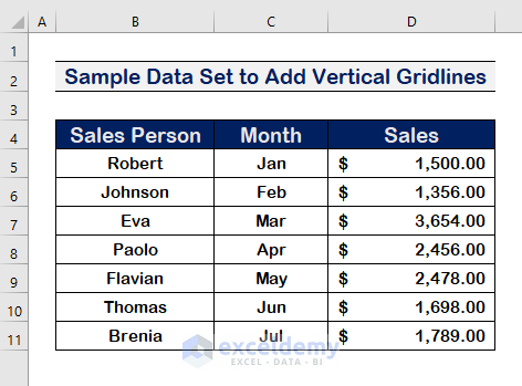
An example data set reflecting the Sales value with the Month for various salespersons is shown in the figure below. We’ll make a chart that shows Sales vs. Months and add vertical gridlines to it. To add the vertical gridlines, we will use two methods: the Chart Element Button and the Chart Tools Menu.
1. Apply the Chart Elements Button to Add Vertical Gridlines to Excel Chart
First of all, we need to make a chart with the Months and Sales Value. To do so, follow the simple steps below.
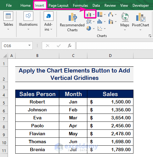
Step 1: Insert a Chart
- Firstly, click on the Insert.
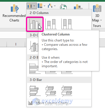
- From the Charts Ribbon, select any chart option you prefer.
Step 2: Add a Chart Layout
- Select a Chart Layout.
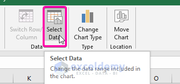
Step 3: Use the Data Ribbon
- Click on the Select Data option to add data to the Chart.
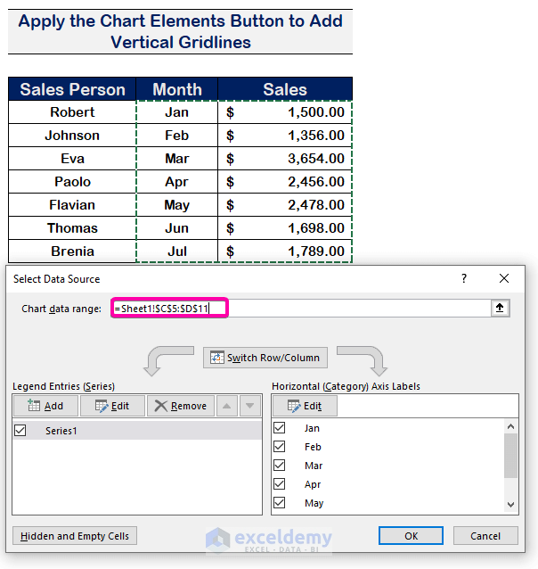
Step 4: Select the Data for the Chart
- Select the data in the image to input the chart data in the Chart data range
- Then, click on OK.
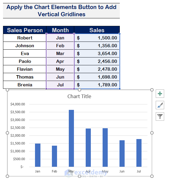
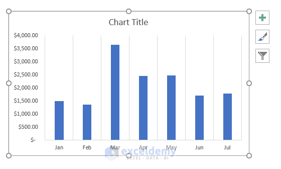
- Therefore, your chart will appear as the image shown below.
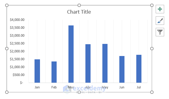
1.1 Add Primary Major Vertical Gridlines
Steps:
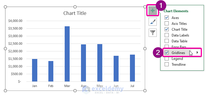
- First, click on the right-side (+) icon to show the Chart Elements.
- Select the Gridlines.
- Then, select the Primary Major Vertical option to add major vertical gridlines.
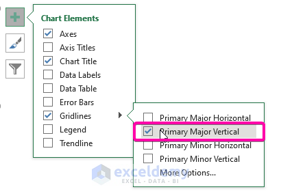
- Therefore, your Primary Major Vertical lines will show in the image shown below.
1.2 Add Primary Minor Vertical Gridlines
Steps:
- From the Gridlines option, select the Primary Minor Vertical.
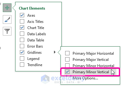
- As a result, the Primary Minor Vertical lines will show up like this.
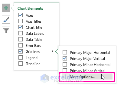
1.3 Format the Gridlines
Steps:
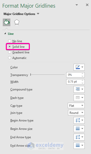
- To Format or add more options, click on More Options.
- To add a solid vertical line, select the Solid Line.
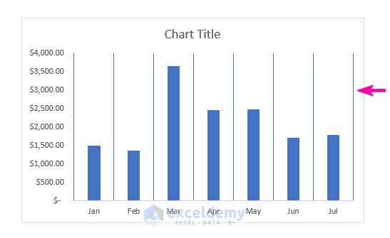
- The solid vertical lines are added in this manner, as demonstrated in the figure below.
- To add gradient lines, select the Gradient line.
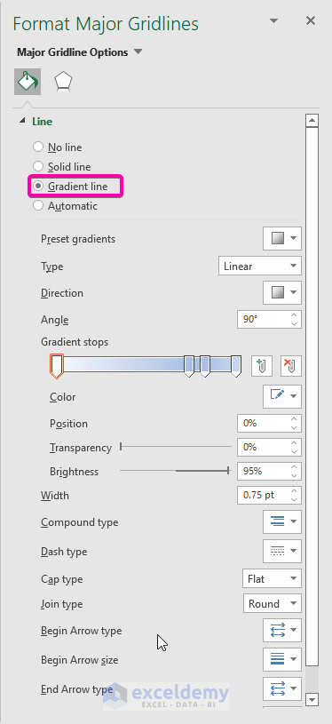
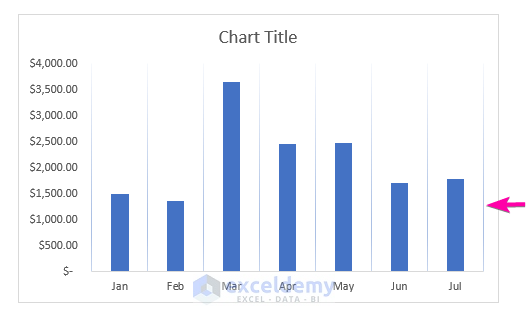
- Adding a Gradient line will result in the chart displayed in the image below.
2. Use the Chart Tools Menu to Add Vertical Gridlines to Excel Chart
Besides the Chart Elements option, we can use the Chart Tools menu to add vertical gridlines. Follow the outlined instructions below to apply the Chart Tools menu.
Step 1: Add Primary Major Vertical Gridlines
- First, click on the Chart Design.
- Select the Add Chart Element.
- Then, select Gridlines.
- Finally, choose the Primary Major Vertical.
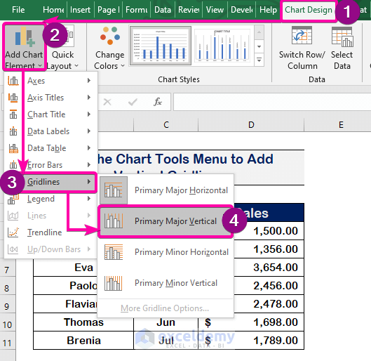
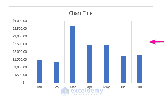
- Therefore, you will get the Primary Major Vertical.
Step 2: Add Primary Minor Vertical Gridlines
- From the Gridlines option, choose the Primary Minor Vertical.
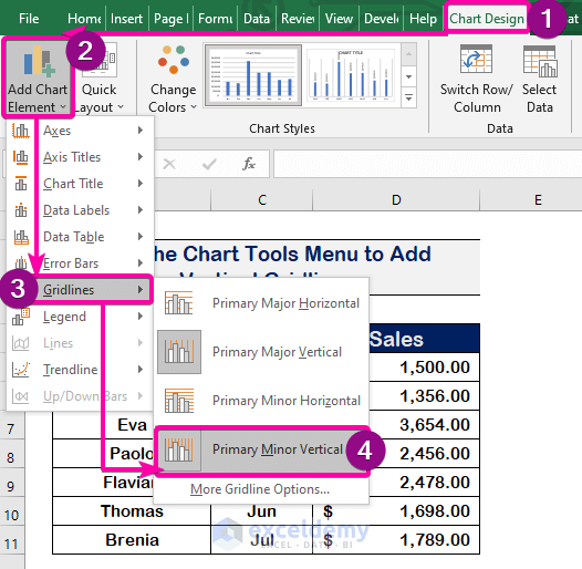
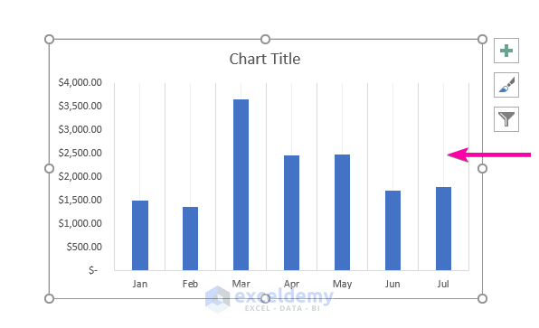
- As a result, after adding the Minor Vertical lines, your chart will display as the image shown below.
Download Practice Workbook
Download this practice workbook to exercise while you are reading this article.
Conclusion
To conclude, I hope this article has given you some useful information about how to add vertical gridlines to an Excel chart. All of these procedures should be learned and applied to your dataset. Take a look at the practice workbook and put these skills to the test. We’re motivated to keep making tutorials like this because of your valuable support.
If you have any questions – Feel free to ask us. Also, feel free to leave comments in the section below.
Related Articles
- How to Add Primary Major Horizontal Gridlines in Excel
- How to Add Primary Minor Vertical Gridlines in Excel
- How to Add Minor Gridlines in Excel
- How to Add Gridlines to a Graph in Excel
- How to Adjust Chart Gridlines Spacing in Excel
- How to Make Square Grid Lines in Excel Graph
- How to Adjust Gridlines in Excel Chart
- How to Remove Gridlines in Excel Graph
<< Go Back To Gridlines in Excel Chart | Excel Chart Elements | Excel Charts | Learn Excel
Get FREE Advanced Excel Exercises with Solutions!
