Example 1 – Assigning Letter Grades in a Mark Sheet Through a Range Lookup with the Excel VLOOKUP Function
The generic formula of the VLOOKUP function is:
=VLOOKUP(lookup_value, table_array, col_index_num, [range_lookup])
Here, the fourth argument ([range_lookup]) of the VLOOKUP function has to be assigned with TRUE (1) or FALSE (0). TRUE or 1 indicates Approximate Match, whereas FALSE or 0 denotes Exact Match. If you don’t use this optional argument, the function will work with the default input: TRUE.
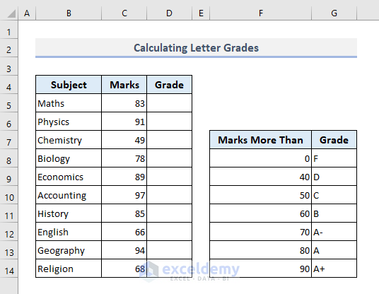
We’ll determine letter grades for several subjects in a final exam. In the following picture, the table on the right represents the grading system. We’ll assign letter grades for all subjects based on the grading system table. We will have to use TRUE or 1 (Approximate Match) for the lookup range argument. We can’t use exact match here since the random marks will not perfectly align with the limits of each grade.
Steps:
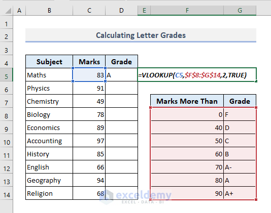
- Select Cell D5 and insert the following:
=VLOOKUP(C5,$F$8:$G$14,2,TRUE)- Press Enter.
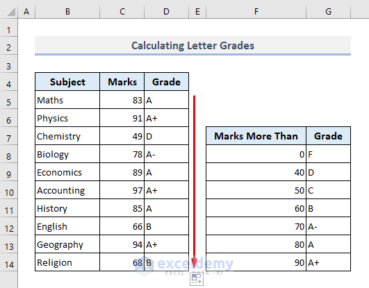
- Use the Fill Handle to autofill the rest of the cells in Column D.
Note: The lookup table data must be in ascending order. Otherwise, the approximate match criteria won’t work properly.
Read More: How to Use Column Index Number Effectively in Excel VLOOKUP Function
Method 2 – Calculating a Discount Based on the Price Range by Applying a Range Lookup with VLOOKUP
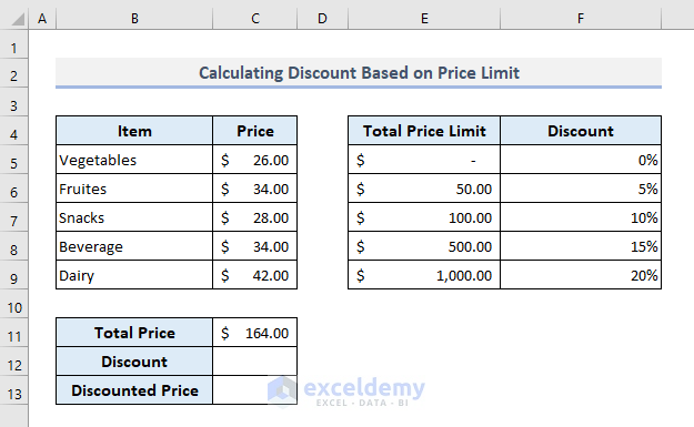
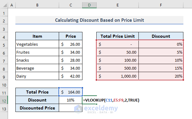
In the following picture, the table on the top left represents some items along with their prices, which will be summed. The table on the right shows the discount system based on the total price limits. By using the discount system table, we’ll find the discount as well as a total discounted price.
Steps:
- Select Cell C12 and copy the following formula inside:
=VLOOKUP(C11,E5:F9,2,TRUE)- Press Enter and the function will return the discount.
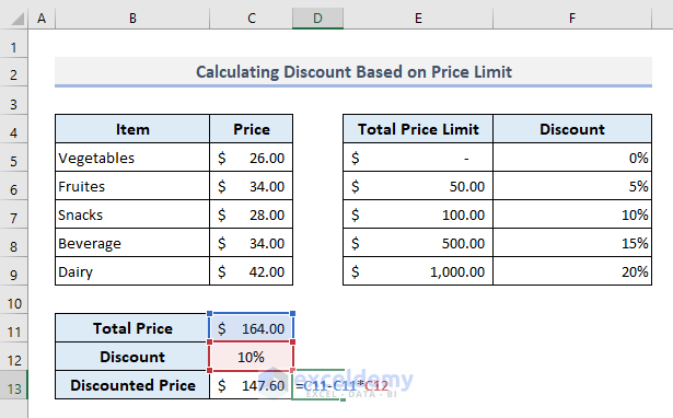
- To calculate the discounted price in Cell C13, apply the following formula:
=C11-C11*C12- Press Enter.
Read More: How to Use VLOOKUP to Find a Value That Falls Between a Range
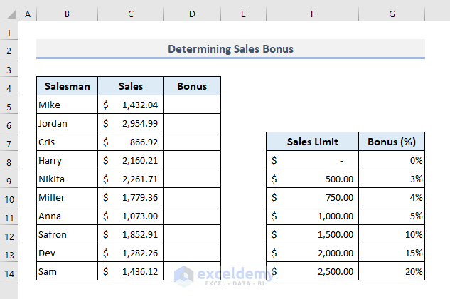
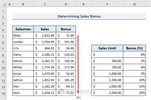
Method 3 – Determining a Sales Bonus by Using a Range Lookup in Excel via VLOOKUP
In the following picture, the table on the right represents the bonus system. In Column D, we’ll directly calculate the bonus based on the bonus percentage and sales value for each salesperson.
Steps:
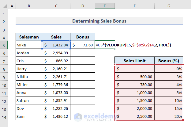
- Select the cell D5 and copy the following formula in it:
=C5*(VLOOKUP(C5,$F$8:$G$14,2,TRUE))- Press Enter to get the first result.
Use the Fill Handle to autofill the rest of the cells in Column D to determine the bonuses for everyone.
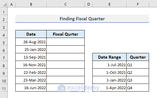
Method 4 – Finding Fiscal Quarters from Dates by Using a Range Lookup with VLOOKUP
We’ll determine a fiscal quarter for a date and assign it with a value Q1, Q2, Q3, or Q4. Let’s assume that the fiscal year starts from 1 July 2021 in our dataset which will run through the next 12 months. The table on the right in the picture below represents the fiscal quarter system based on the date range.
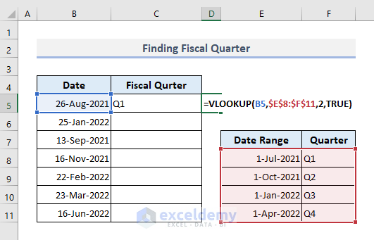
Steps:
- Select Cell C5 and insert the following formula:
=VLOOKUP(B5,$E$8:$F$11,2,TRUE)- Press Enter for the first result.
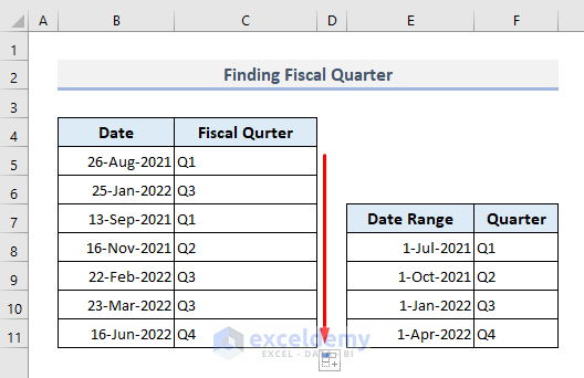
- Autofill the entire Column C to get all other fiscal quarters for the given dates in Column B.
Read More: How to Apply VLOOKUP by Date in Excel
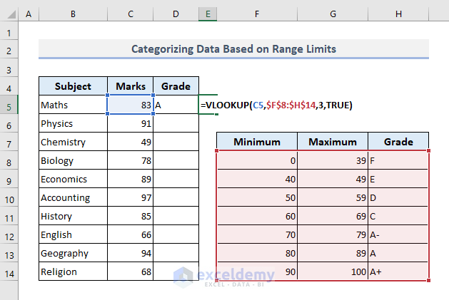
Method 5 – Categorizing Data Based on Range Limits with VLOOKUP
Let’s expand the first example where we had to calculate the grades for several subjects. The table on the right will contain minimum and maximum scores or marks for certain letter grades. Based on this grading system, we’ll assign the letter grades in Column D for all subjects.

Steps:
- Select the output Cell D5 and copy the following formula into it:
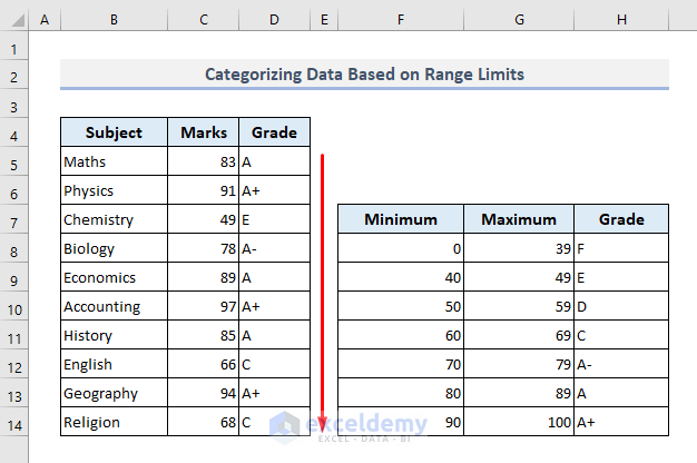
=VLOOKUP(C5,$F$8:$H$14,3,TRUE)- Press Enter to get the first grade.
- Use the Fill Handle to autofill the rest of the cells in Column D to get all other letter grades.
Download Practice Workbook
You can download the Excel workbook that we’ve used to prepare this article.
Further Readings
- How to Use VLOOKUP If Condition Lies Between Multiple Ranges in Excel
- Lookup and Return Value in a Range in Excel (5 Ways)
- How to Find Second Match with VLOOKUP in Excel (2 Simple Methods)

