Revised Schedule 3 Balance Sheet Format in Excel with Formula

Step 1 – Setting Up Balance Sheet Format

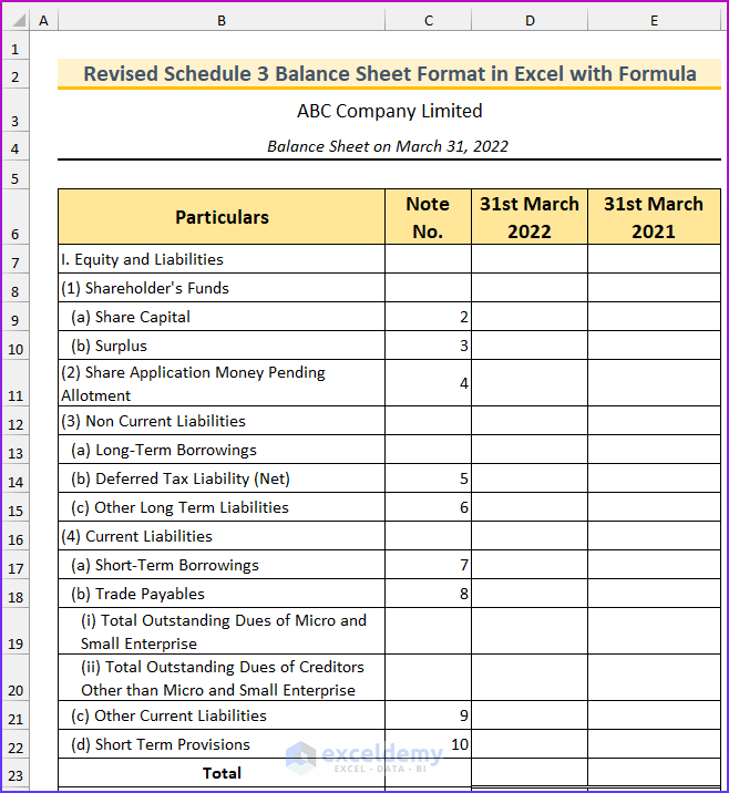
We will specify the balance sheet format according to the revised Schedule 3 in Excel with the formula. The example company name is “ABC Company Limited,” and this is a Division I company. We are creating the balance sheet for March 31, 2022, as the Indian fiscal year starts on April 1.

• Type the following fields on the spreadsheet.
• Add the note numbers which we will input in the second step.
• We will add two columns for this year and the last year.
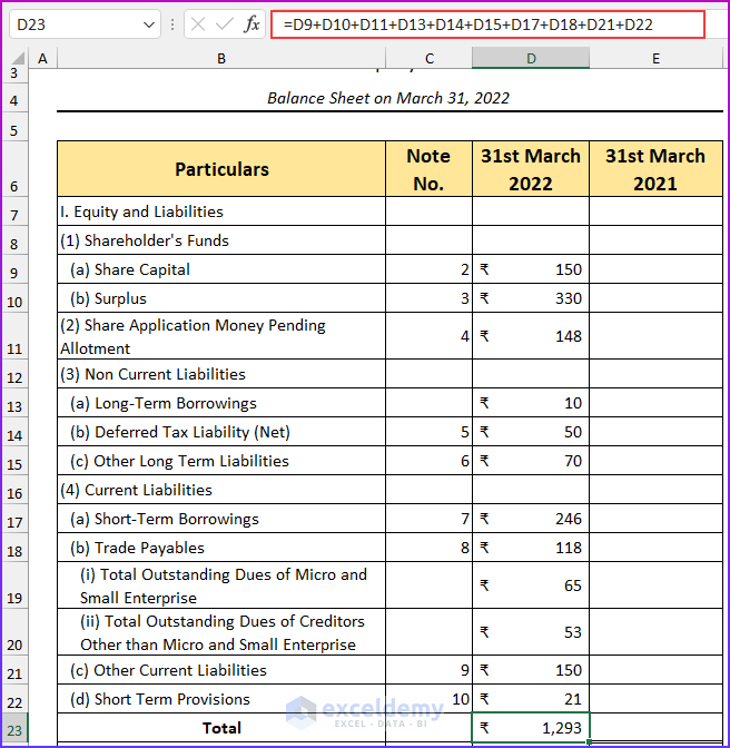
• In the following image, you can see the equity and liabilities part of the balance sheet.

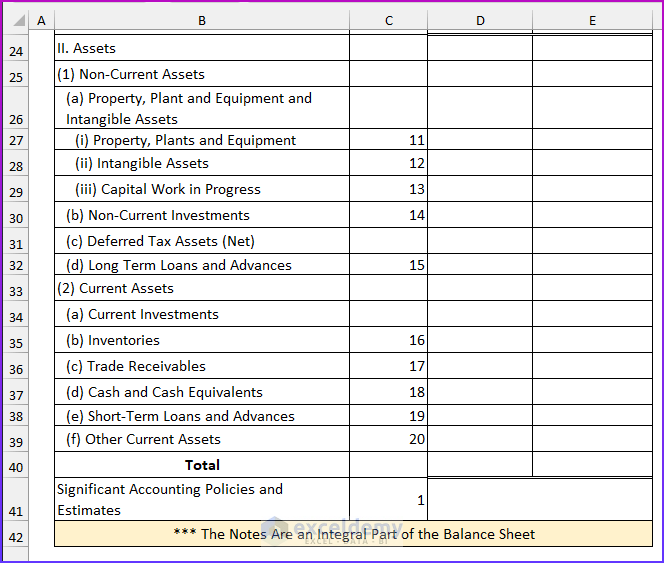
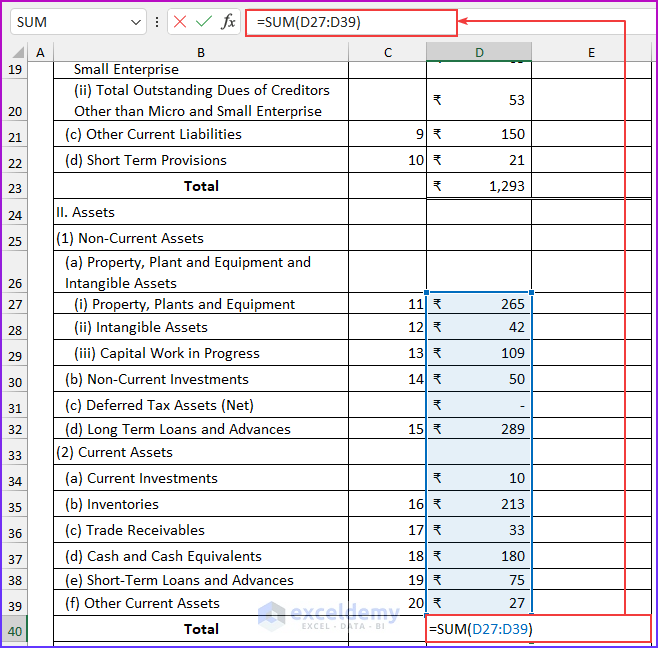
• Input the assets part of the balance sheet.

Read More: How to Create Tally Debit Note Format in Excel

Step 2 – Entering Note Details

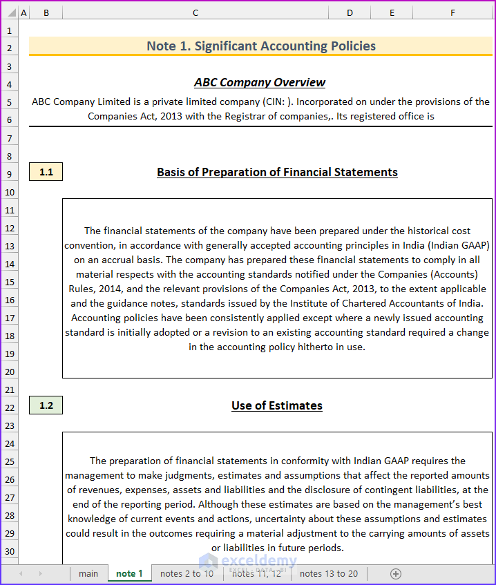
There are twenty notes for the revised Schedule 3 balance sheet format. The first note is for the company’s accounting policies. Then, the next nine notes are for the equity and liability parts. Finally, the last 10 notes are for the assets part of the balance sheet.

• Type the company accounting policies in the “note 1” sheet.

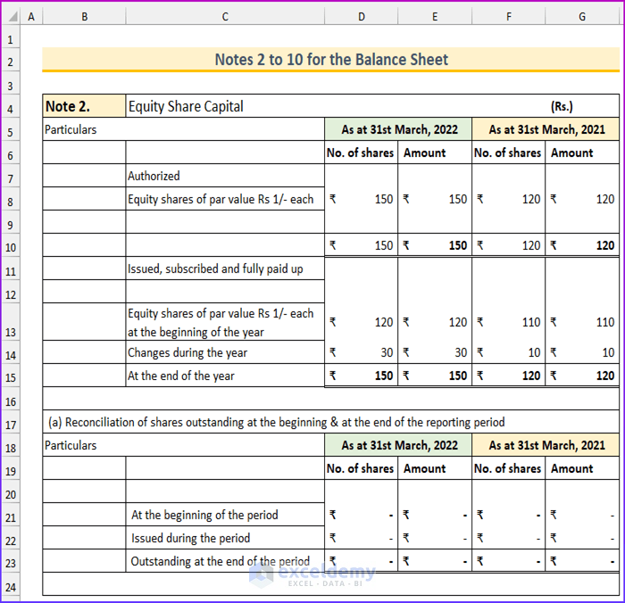
• Type the details of note 2 for the equity share capital. Here the values are inserted randomly.

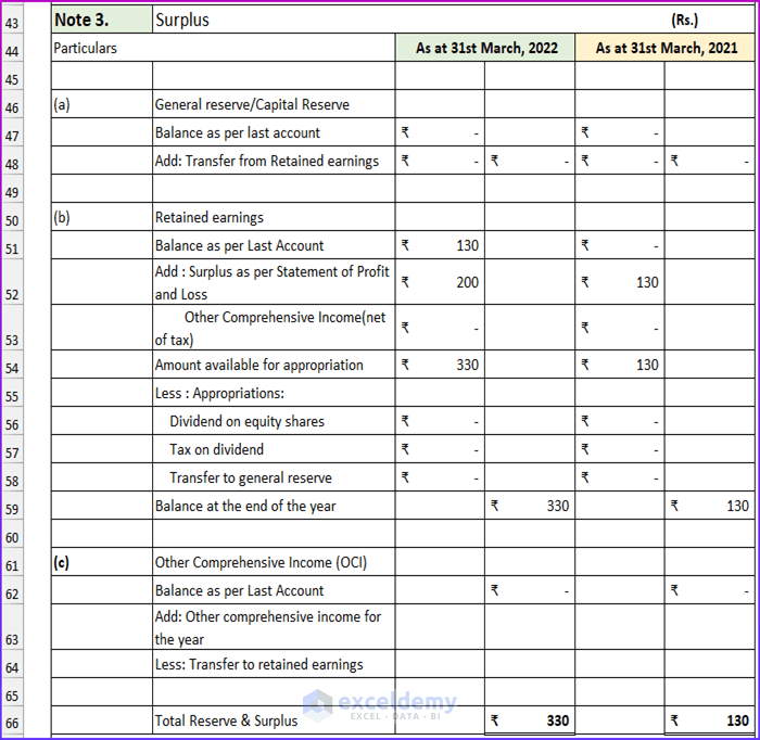
• Input the details of note 3 for the surplus.

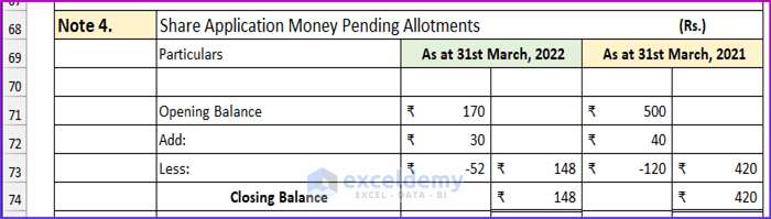
• Input the details of the share application money pending allotments.

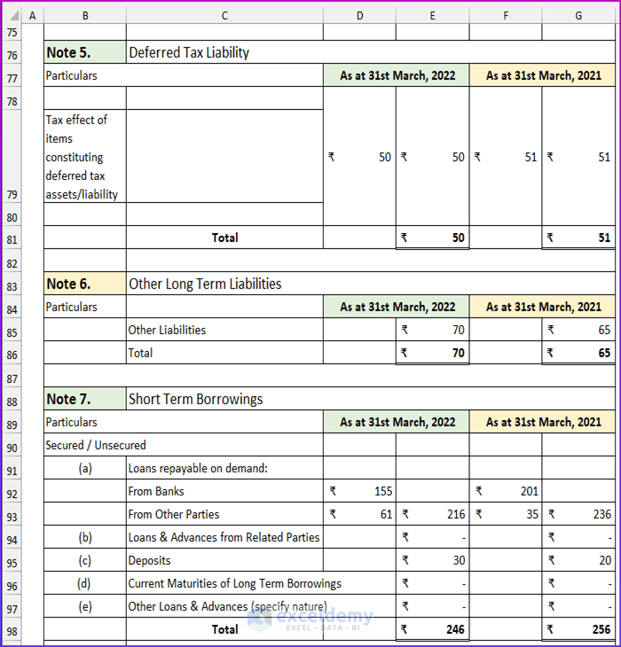
• Put the values for notes 5, 6, and 7.

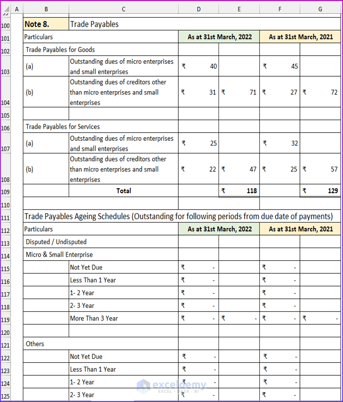
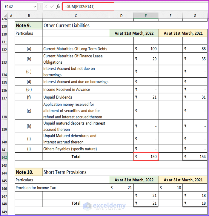
• Input the details for note 8.

• Copy the following formula to find the total values of other current liabilities.

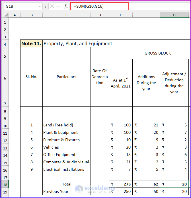
• Type the details for note 10.

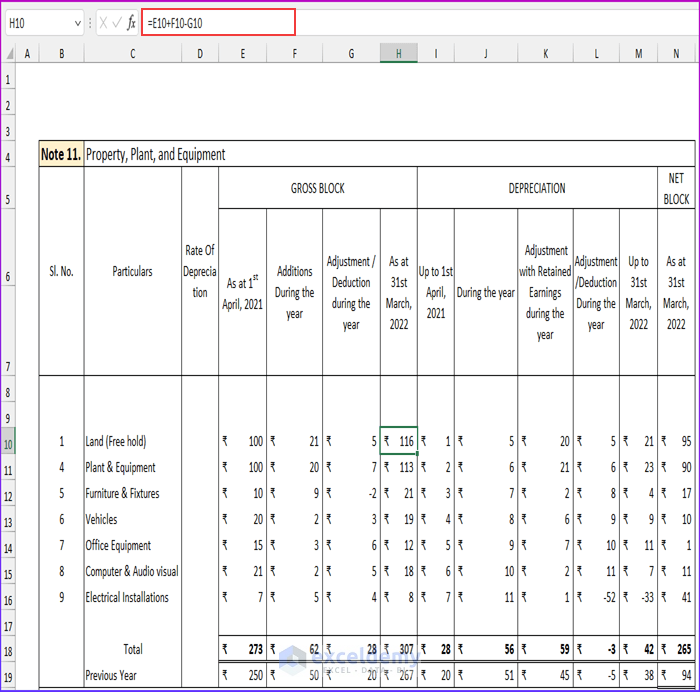
• Input the following formula to find the value of the total gross block:

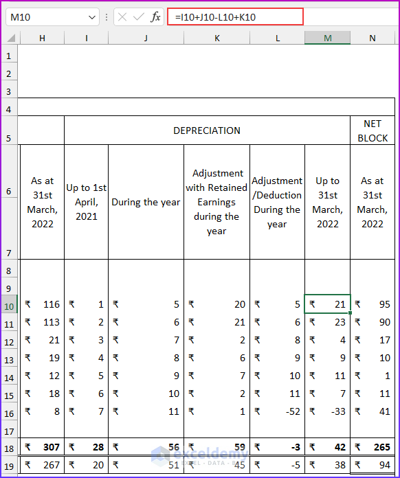
• Input this formula to calculate the value of depreciation:

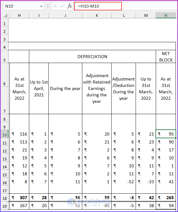
• Input this formula to find the value of the netblock:

• Input the following formula to return the total amount. Additionally, type the previous year’s values.

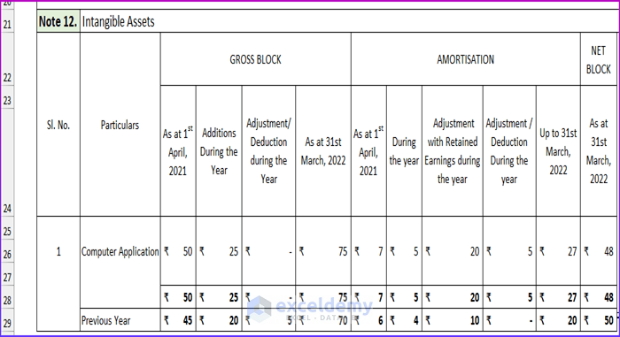
• Type the details for note 12.

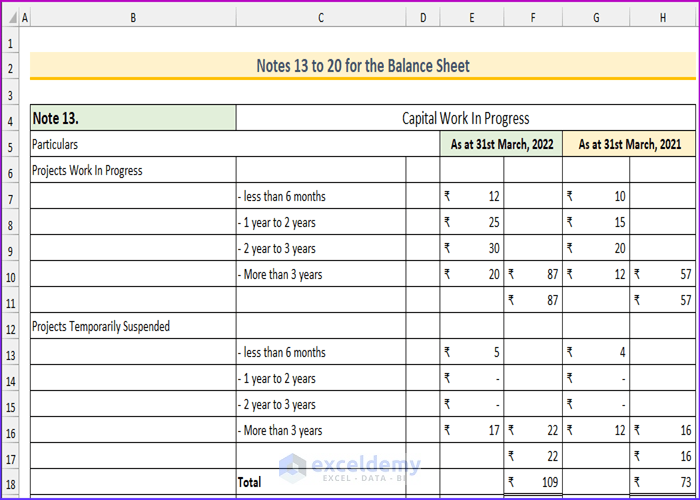
• Type the following values to complete note 13.

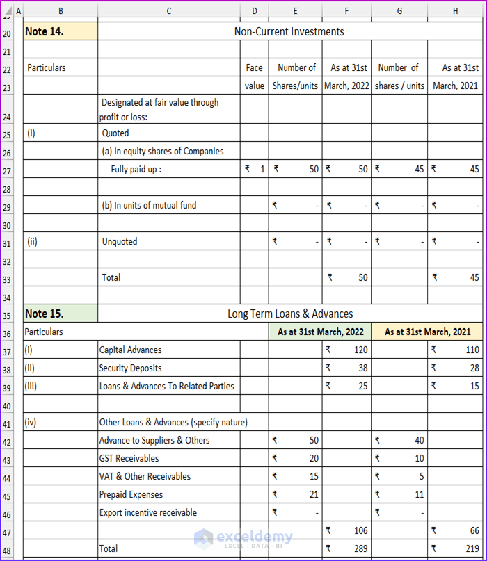
• Type the details for notes 14 and 15.

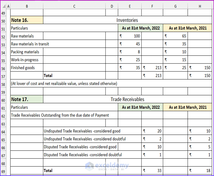
• Input values to complete notes 16 and 17.

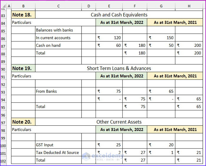
• Finish with the rest of the notes.

Read More: Balance Sheet Format in Excel with Formulas

Step 3 – Linking Notes to Balance Sheet

• Link the values for the share capital from the “notes 2 to 10” sheet. In the formula bar, we can see the following formula:

• Link the values from the notes to the rest of the values in the balance sheet.
• Copy the following formula in cell D23 to find the total values of equity and liability.

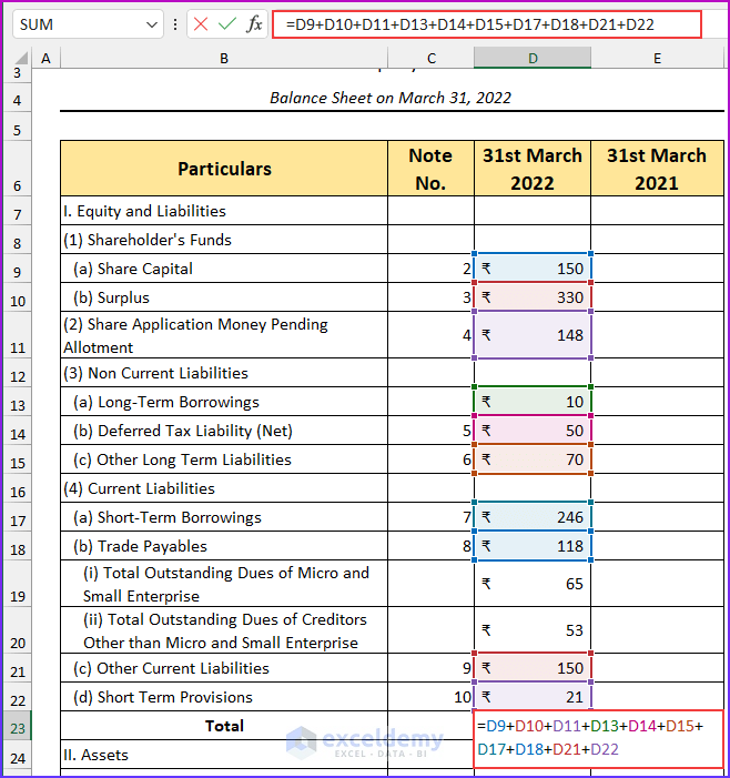
• Press Enter and it will return the total value.

• Enter this formula in cell D40 to calculate the value of the total assets.

• Press Enter and we can see that the balance sheet balances.

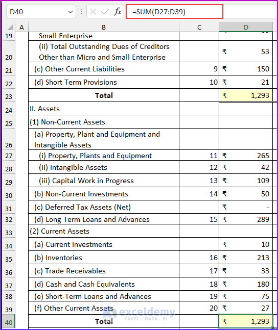
• Complete the values for the year 2021 and the final output will look similar to this snapshot. Here, we have hidden some rows for better visualization.

Read More: Schedule 6 Balance Sheet Format in Excel

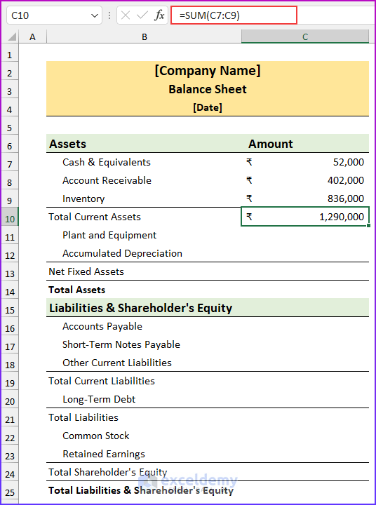
Basic Balance Sheet Format in Excel

Steps:

• Type the following details to create the balance sheet format.
• Insert the relevant values and copy this formula to find the value of total current assets:

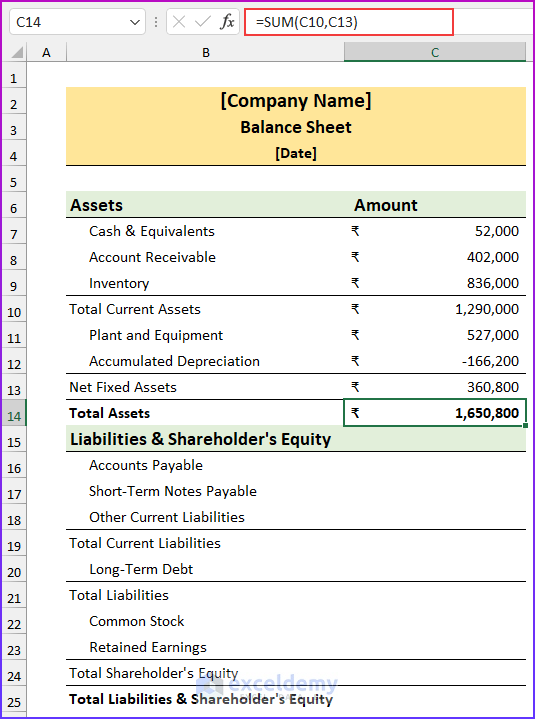
• Copy the following formula to find the values of the total assets.

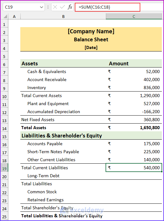
• Use this formula to return the total current liabilities:

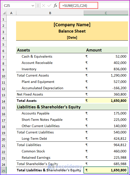
• Put this formula in cell C25 to calculate the values of total liabilities and shareholder’s equity.

Read More: How to Create Vertical Balance Sheet Format in Excel

Things to Remember

• This balance sheet format in Excel based on the revised Schedule 3 should be used as a practice tool. This should not be the basis for your financial records. You should consult with a chartered accountant after preparing the balance sheet.
• The values are in crores and arbitrary.

Download Practice Workbook

You can download the Excel file from the link below.

<< Go Back to Balance Sheet | Finance Template | Excel Templates