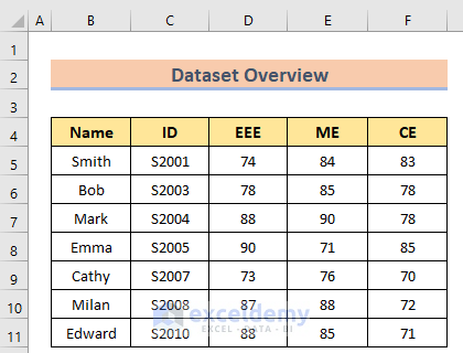
This is the sample dataset.
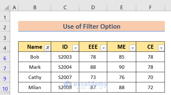
Method 1 – Using the Filter Option
Steps:
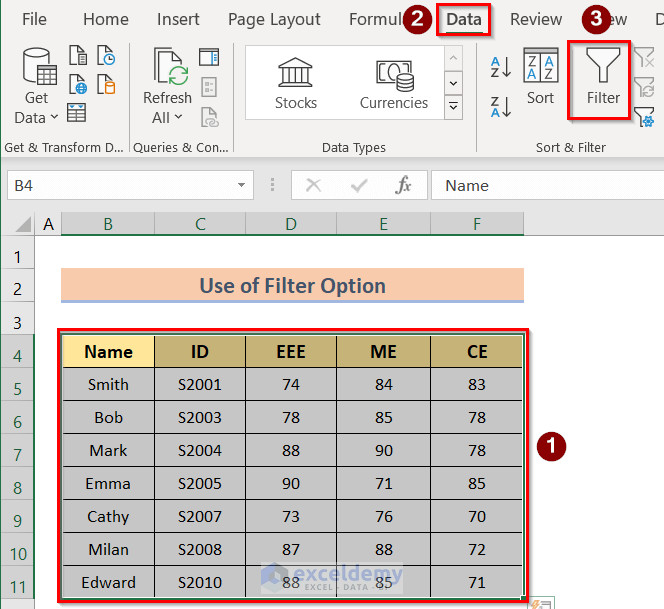
- Go to select the table > Data > Filter.
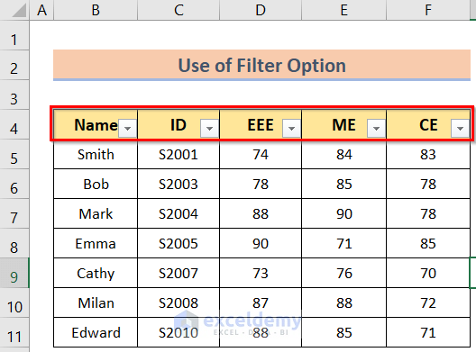
- This is the output.
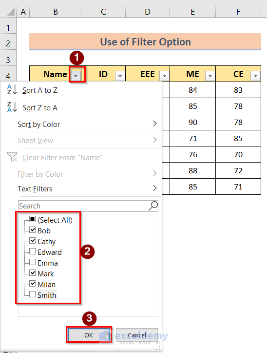
- Click the filter point (Name, here), untick data you don’t want to filter and click OK.
- This is the output.
Read More: How to Skip Hidden Cells When Pasting in Excel
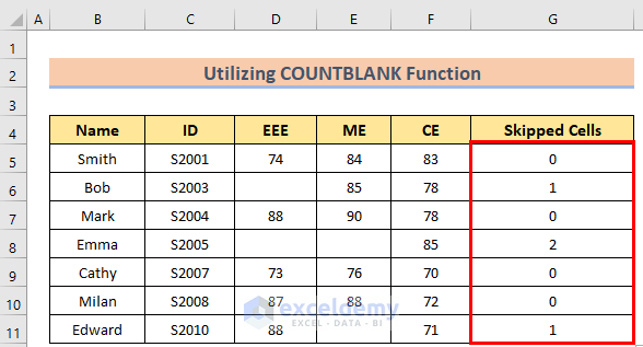
Method 2 – Utilizing the COUNTBLANK Function
Steps:
- Create a dataset.
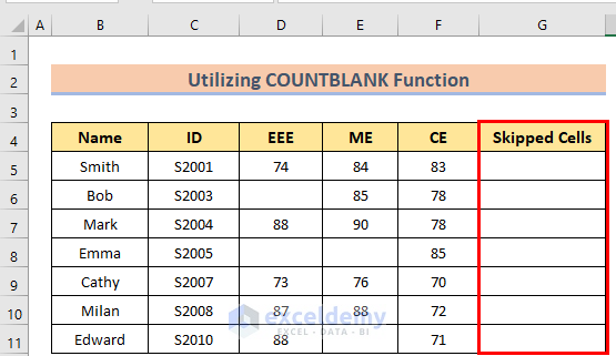
- Enter the following formula in G5.
=COUNTBLANK(B5:F5)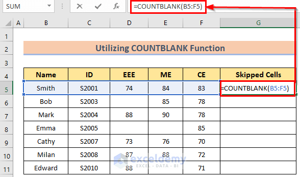
- You will get the results for that cell.
- Drag the Fill Handle across the cells you want to fill.
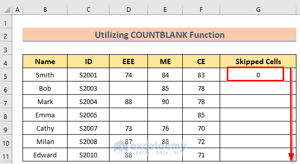
- This is the output.
- Go to select the table > Data > Filter
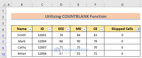
- Click the filter point, untick data you don’t want to filter and click OK.
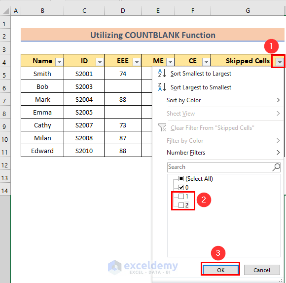
- This is the output.
Read More: How to Skip to Next Cell If a Cell Is Blank in Excel
Method 3 – Using the FILTER Function
Steps:
- Create a dataset.
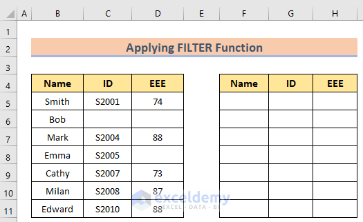
- Enter the following formula in F5.
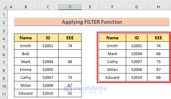
=FILTER(B5:D11,(B5:B11<>"")*(C5:C11<>"")*(D5:D11<>""))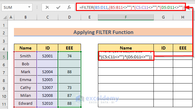
- Press Enter to see the output.
Read More: Skip Cells When Dragging in Excel
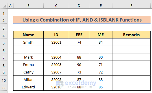
Method 4. Combining the IF, AND & ISBLANK Functions
Steps:
- Create a dataset.
- Enter the following formula in F5.
=IF(AND(ISBLANK(B5), ISBLANK(C5),ISBLANK(D5),ISBLANK(E5)),"Blank", "Not-Blank")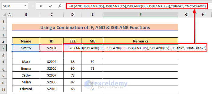
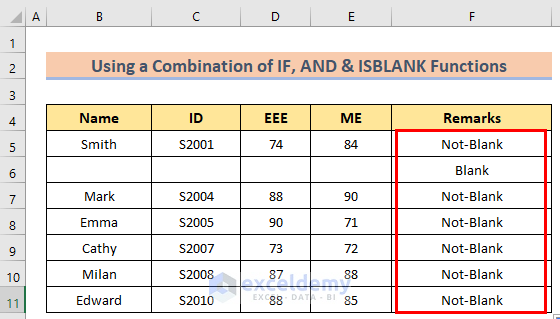
- Drag the Fill Handle across the cells you want to fill.
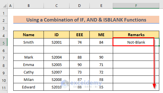
- This is the output.
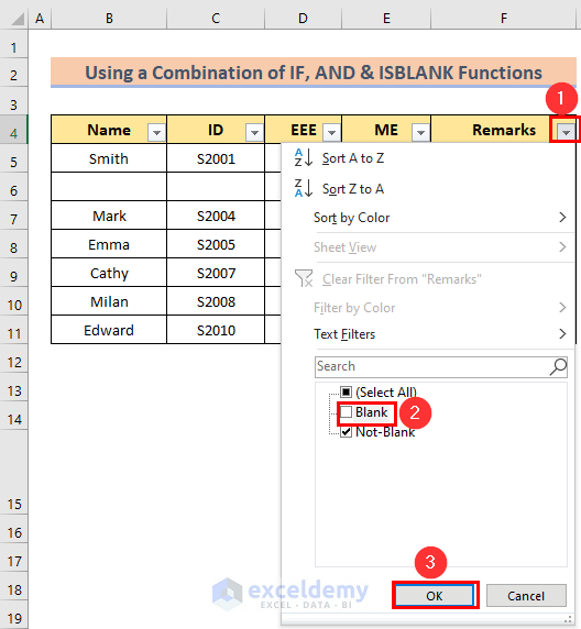
- Go to select the table > Data > Filter
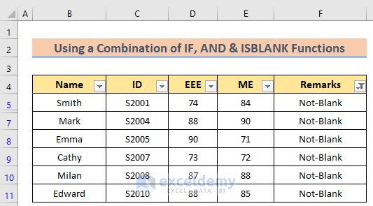
- Click the filter point, untick data you don’t want to filter and click OK.
- Press Enter button to see the output.
Formula Breakdown
- ISBLANK(E5)): refers to the selected cell (E5).
- AND(ISBLANK(B5), ISBLANK(C5), ISBLANK(D5), ISBLANK(E5)), “Blank”, “Not-Blank”: refers to the cell in which conditions will be applied.
- IF(AND(ISBLANK(B5), ISBLANK(C5),ISBLANK(D5),ISBLANK(E5)),”Blank”, “Not-Blank”): Refers to the condition.
Read More: Skip to Next Result with VLOOKUP If Blank Cell Is Present
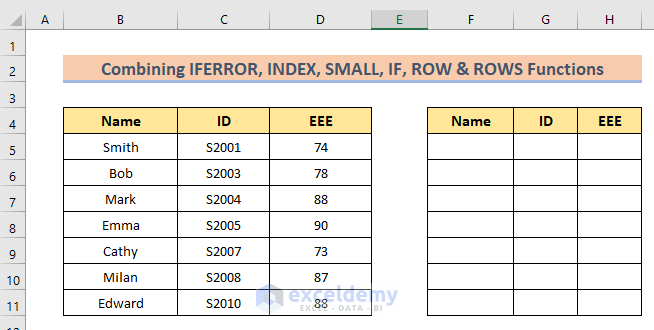
Method 5 – Combining the IFERROR, INDEX, SMALL, IF, ROW & ROWS Functions
Steps:
- Create a dataset.
- Enter the following formula in F5.
=IFERROR(INDEX(B:B,SMALL(IF(B$5:B$11<>"",ROW(B$5:B$11)), ROWS(B$5:B5))), "")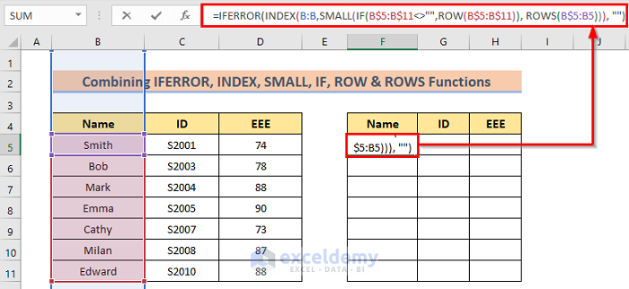
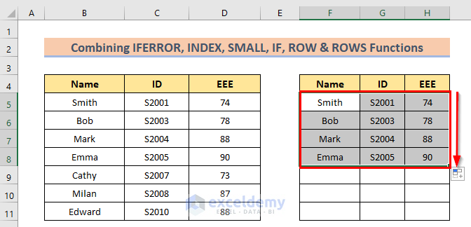
- Press Enter to see the output.
Formula Work Breakdown
- ROWS(B$5:B5): is the reference cell.
- ROW(B$5:B$11): is the selected range.
- SMALL(IF(B$5:B$11<>””,ROW(B$5:B$11)), ROWS(B$5:B5): refers to fixed reference cells.
- IFERROR(INDEX(B:B,SMALL(IF(B$5:B$11<>””,ROW(B$5:B$11)), ROWS(B$5:B5))), “”): is the condition.
Read More: How to Skip Lines in Excel
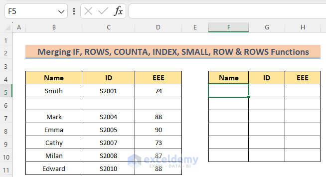
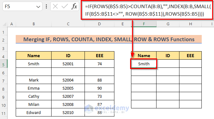
Method 6 – Merging IF, ROWS, COUNTA, INDEX, SMALL, ROW & ROWS Functions
Steps:
- Create a dataset.
- Enter the following formula in F5.
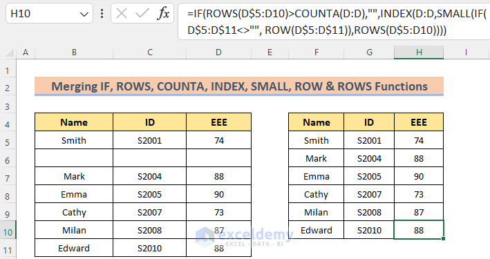
=IF(ROWS(B$5:B5)>COUNTA(B:B),"",INDEX(B:B,SMALL(IF(B$5:B$11<>"", ROW(B$5:B$11)),ROWS(B$5:B5))))- Press Enter to see the output.
- Drag the Fill Handle across the cells you want to fill.
Formula Breakdown
- ROWS(B$5:B5): is the reference cell.
- ROW(B$5:B$11): is the selected range.
- INDEX(B:B,SMALL(IF(B$5:B$11<>””, ROW(B$5:B$11)),ROWS(B$5:B5))): is the counta function.
- IF(ROWS(B$5:B5)>COUNTA(B:B),””,INDEX(B:B,SMALL(IF(B$5:B$11<>””, ROW(B$5:B$11)),ROWS(B$5:B5)))): is the condition.
Read More: How to Skip Blank Rows Using Formula in Excel
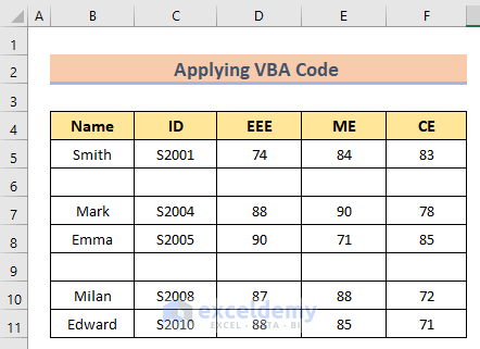
Method 7 – Applying a VBA Code
Steps:
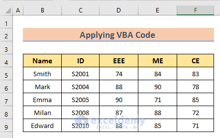
- Create a dataset.
- Press Alt+F11 to open the VBA window.
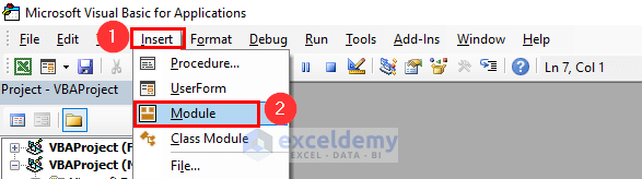
- Enter the following code >> save the VBA code.
Sub Skip_Blank_Rows()
Range("B5:F11").Select
Selection.SpecialCells(xlCellTypeBlanks).EntireRow.Delete
End Sub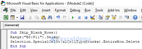
- Click RUN or press F5 to see the output.
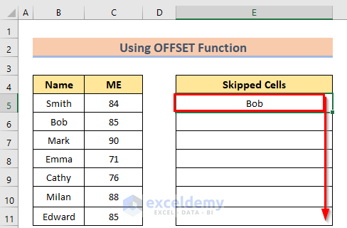
Method 8 – Using the OFFSET Function
Steps:
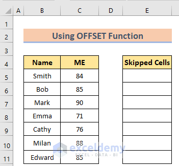
- Create a dataset.
- Enter the following formula in E5.
<span style="font-size: 14pt;">=OFFSET($B$5,ROW(D1)*2-1,0)</span>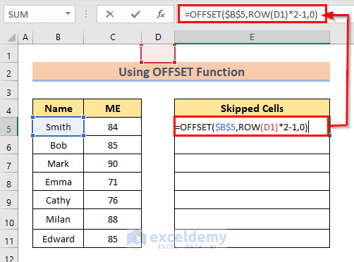
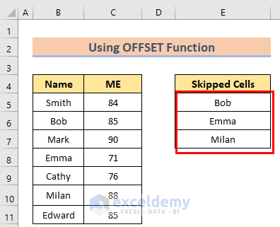
- Press Enter to see the output.
- Drag the Fill Handle across the cells you want to fill.
Download Practice Workbook
Download the practice workbook here.
Related Articles
- How to Skip a Column When Selecting in Excel
- Excel Formula to Skip Rows Based on Value
- How to Skip Every Other Column Using Excel Formula
- How to Skip Columns in Excel Formula
<< Go Back to Skip Cells | Excel Cells | Learn Excel
Get FREE Advanced Excel Exercises with Solutions!
