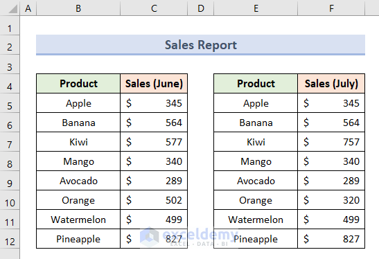
Consider the following dataset example for demonstration. Here the two datasets represent sales information for June and July of 8 products. We will perform a reconciliation of these two datasets to find mismatches.
Method 1 – Use the VLOOKUP Function to Perform a Reconciliation in Excel
- Insert the following VLOOKUP formula in cell H5:
=VLOOKUP(E5,$B$5:$C$12,2,FALSE)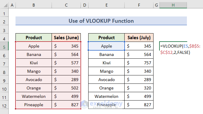
Here, as we are extracting data from the 1st dataset, therefore the column number is 2. FALSE is given to get the exact match.
- Press Enter.
- Insert this formula in cell I5 for the deduction:
=F5-H5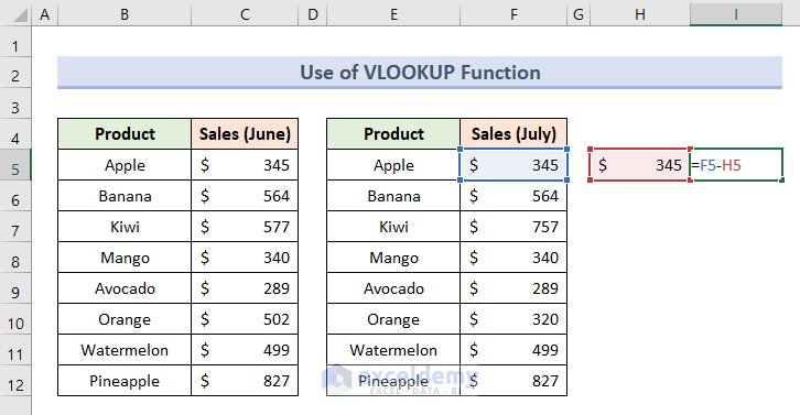
- Hit Enter.
- Use the AutoFill tool to apply the same formulas for other values.
- You can see that the variation between the two datasets is visible.
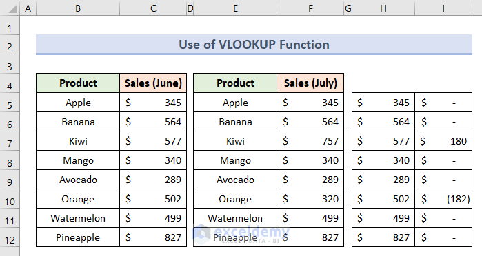
Negative values in the Accounting format are presented in parentheses.
Read More: How to Reconcile Two Sets of Data in Excel
Method 2 – Reconciliation with INDEX-MATCH Functions
- Insert the following formula in cell H5:
=INDEX($C$5:$C$12,MATCH(E5,$B$5:$B$12))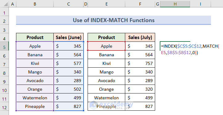
- Press Enter.
- Insert this formula to get the deducted value in cell I5:
=F5-H5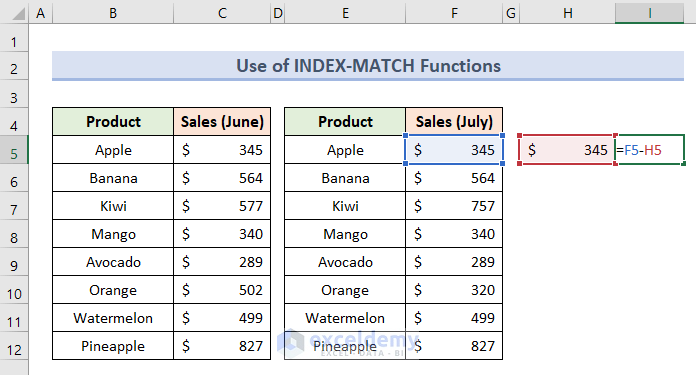
- Press Enter.
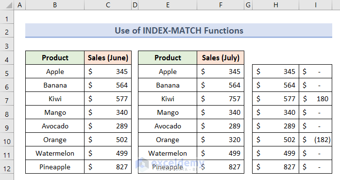
- Apply AutoFill for the cell range H6:I12.
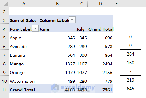
Method 3 – Apply a Pivot Table for Reconciliation
- Combine two datasets into one.
- Since the datasets are for two different months, make a new column for the month.
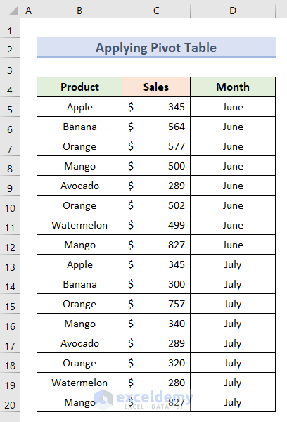
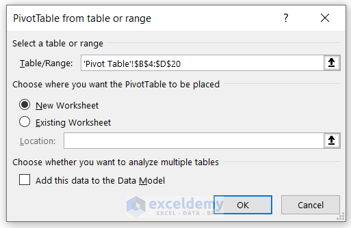
- Select the cell range B4:D20.
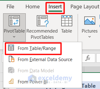
- Go to the Insert tab and select Pivot Table.
- Choose the option From Table/Range.
- In the new dialogue box, you can see the cell range is showing to create a pivot table.
- Press OK.
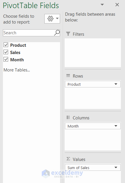
- A new Pivot Table Fields panel appears.
- Place the columns named Product, Month and Sales inside the Rows, Columns and Values category, respectively.
- Insert this formula in cell F5 in the same worksheet as the new pivot table.
=B5-C5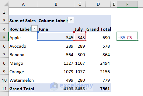
- Hit Enter.
- Use the AutoFill tool to apply the same formula for the entire data series.
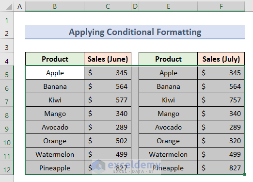
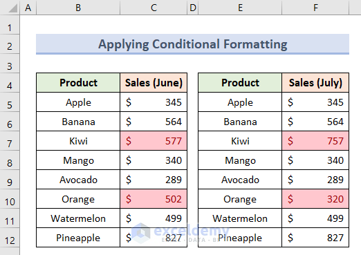
Method 4 – Apply Conditional Formatting for Reconciliation
- Select the cell range B5:F12.
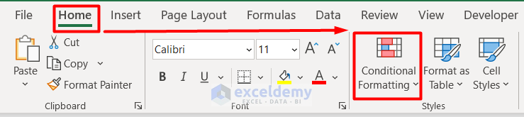
- Go to the Home tab and click on Conditional Formatting.
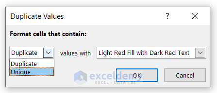
- Select Highlight Cells Rules and choose Duplicate Value from the drop-down.
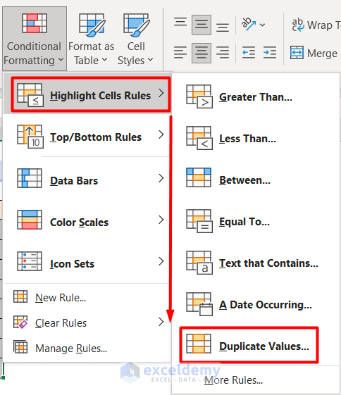
- Select the condition Unique and press OK.
- You can see the different values are marked.
Read More: How to Perform Bank Reconciliation Using VLOOKUP in Excel
Method 5 – Insert a MATCH Function for Reconciliation
- Insert this formula in cell H5:
=ISNUMBER(MATCH(F5:F12,$C$5:$C$12,0))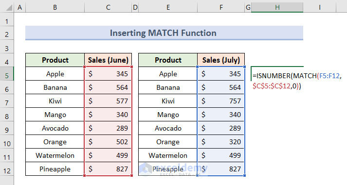
Here, the ISNUMBER function denotes the value, while the MATCH function compares dynamic arrays between two datasets. Lastly, insert 0 for the exact match.
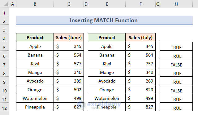
- Press Enter (or Ctrl + Shift+ Enter).
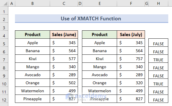
Method 6 – Reconcile with the XMATCH Function in Excel
- Insert this formula in cell H5:
=NOT(ISNUMBER(XMATCH(F5:F12,C5:C12)))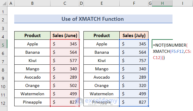
Here, The ISNUMBER function returns TRUE when a cell contains a number, and FALSE if not. This is why the NOT function is used at the beginning to get an exact match. The XMATCH function searches for the specific item among the selected cells.
- Press Enter.
- You will get the reconciliation output for all the values.
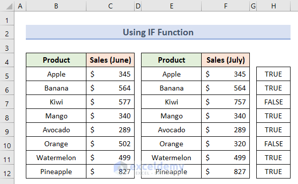
Method 7 – Use the IF Function for Reconciliation
- Insert this formula in cell H5.
=IF(C5=F5,"TRUE","FALSE")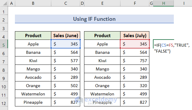
Here, the IF function compares the selected cells on the condition of true or false.
- Hit Enter.
- Use AutoFill to drag the formula in cell range H6:H12.
Method 8 – Apply the COUNTIF Function for Reconciliation in Excel
- Insert this formula in cell H5.
=IF(COUNTIF(C5:C12,F5:F12)<>0,"True","False")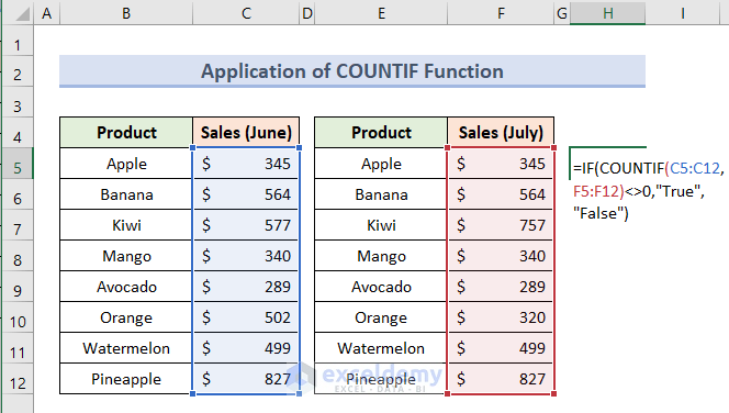
Here, the COUNTIF function counts the number of times a value, or text is contained within a range.
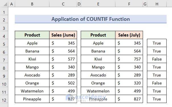
- Hit Enter.
Read More: How to Reconcile Data in Excel
Method 9 – Reconcile Datasets with the XLOOKUP Function
- Insert this formula in cell H5.
=ISTEXT(XLOOKUP(E5,$B$5:$B$12,$B$5:$B$12))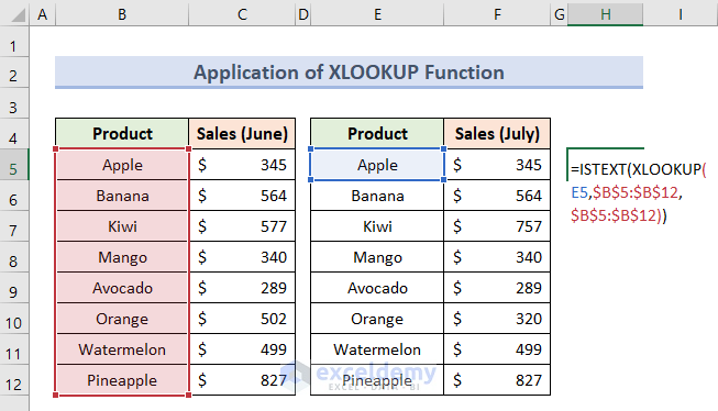
Here, the XLOOKUP will return a corresponding value from a cell, and you can define a result if the value is not found. The ISTEXT function will fetch the texts from the dataset.
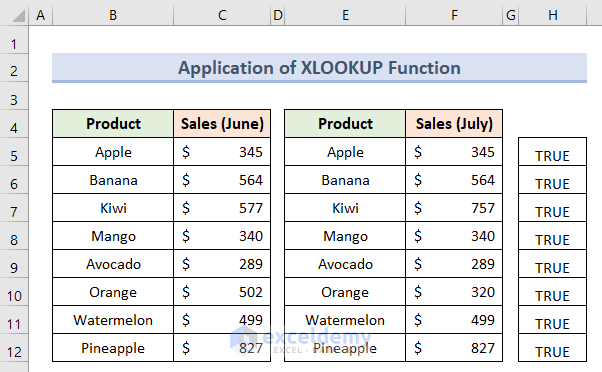
- Press Enter.
- Use the AutoFill tool to drag the formula to cell range H6:H12.
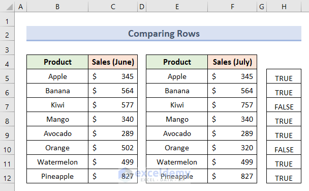
Method 10 – Comparing Rows for Reconciliation of Datasets in Excel
- Put this formula in cell H5.
=C5=F5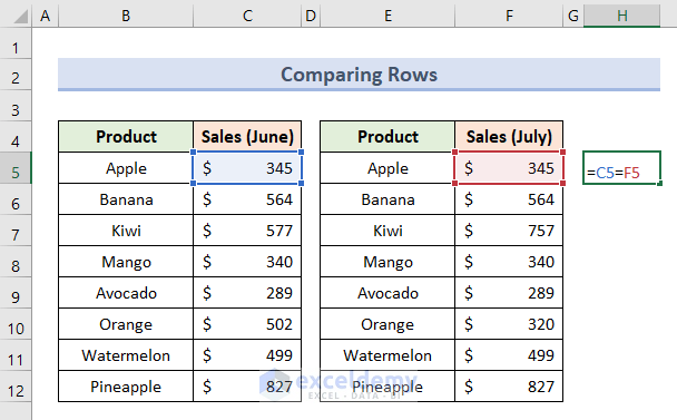
- Hit Enter.
- Drag the bottom corner of cell H5 up to cell H12.
- You can see the compared results.
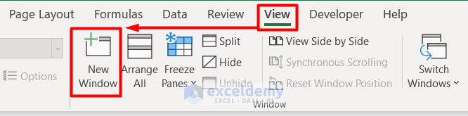
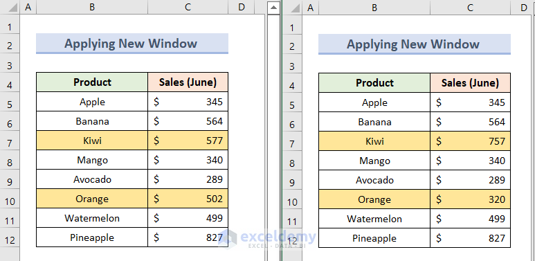
Method 11 – Apply the New Window Option for Reconciliation in Excel
- Go to the View tab in worksheet Dataset 1.
- Choose New Window.
- You will get a copy of the similar workbook.
- Go to the Dataset 2 worksheet.
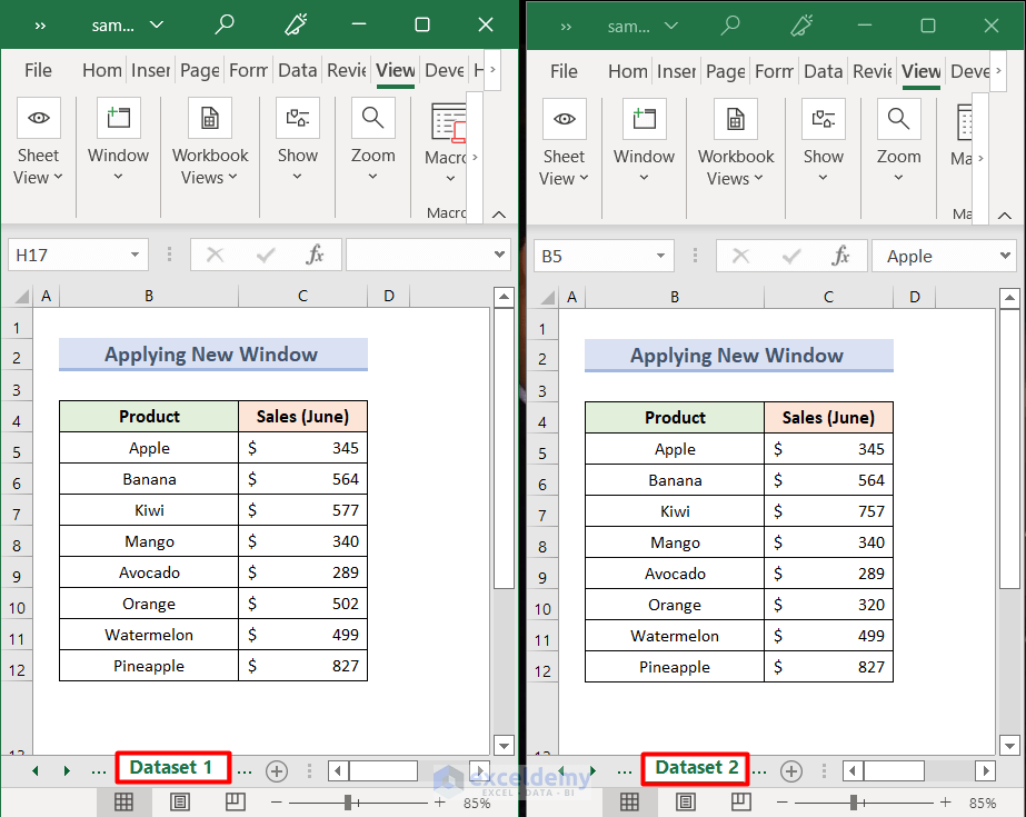
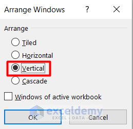
- In the Dataset 1 worksheet, go to the Home tab again and select Arrange All.

- In the Arrange Windows dialogue box, select Vertical.
- Press OK.
- You can view the worksheets simultaneously and highlight differences among them.
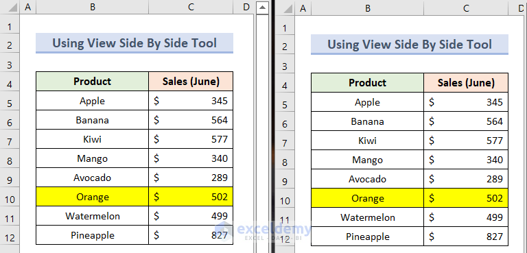
Method 12 – Use the View Side by Side Tool to Reconcile Two Workbooks
- Go to the View tab.
- Select View Side by Side under the Window group.
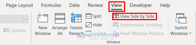
- You will see the other workbook in parallel.
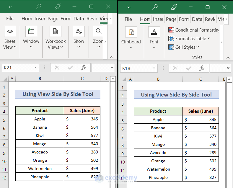
- You can compare the datasets and highlight the differences like this:
Read More: How to Reconcile Data in 2 Excel Sheets
Download the Workbook
Related Articles
- How to Do Intercompany Reconciliation in Excel
- Automation of Bank Reconciliation with Excel Macros
- How to Reconcile Vendor Statements in Excel
- How to Reconcile Credit Card Statements in Excel
<< Go Back to Excel Reconciliation Formula | Excel for Accounting | Learn Excel
Get FREE Advanced Excel Exercises with Solutions!
