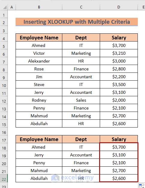
Here’s the overview of using XLOOKUP with multiple criteria.
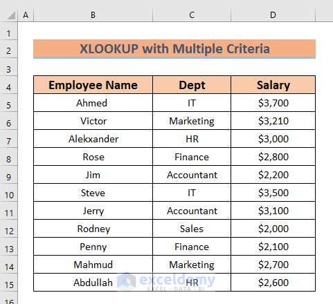
The following dataset has the Employee Name, Dept, and Salary columns. We will extract various data using multiple conditions in the XLOOKUP function.
Method 1 – Using Only the XLOOKUP Function with Multiple Criteria in Excel
Case 1.1 – Using the Ampersand Operator to Set Multiple Criteria
Steps:
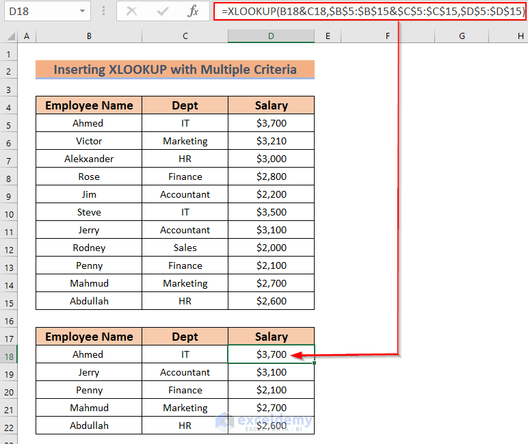
- We selected cell D18.
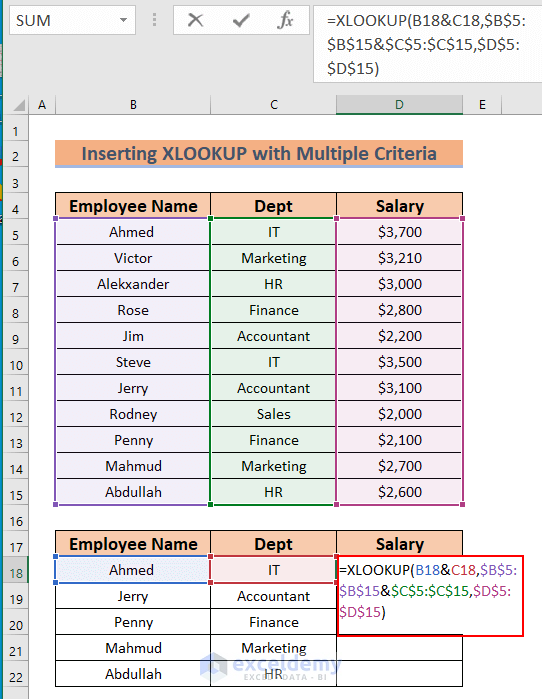
- Use the following formula in the selected cell or into the Formula Bar.
=XLOOKUP(B18&C18,$B$5:$B$15&$C$5:$C$15,$D$5:$D$15)
Formula Breakdown
- We want to look up the Salary of Ahmed who works in the IT department.
- In the function, we selected the lookup_value F4 & G4.
- The lookup_array is B5:B15 & C5:C15.
- We selected the return_array D5:D15.
- Hit Enter. The formula will show the Salary of the given lookup_value.
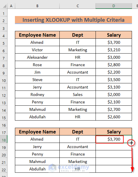
- Use the Fill Handle to AutoFill the formula for the rest of the cells in the column.
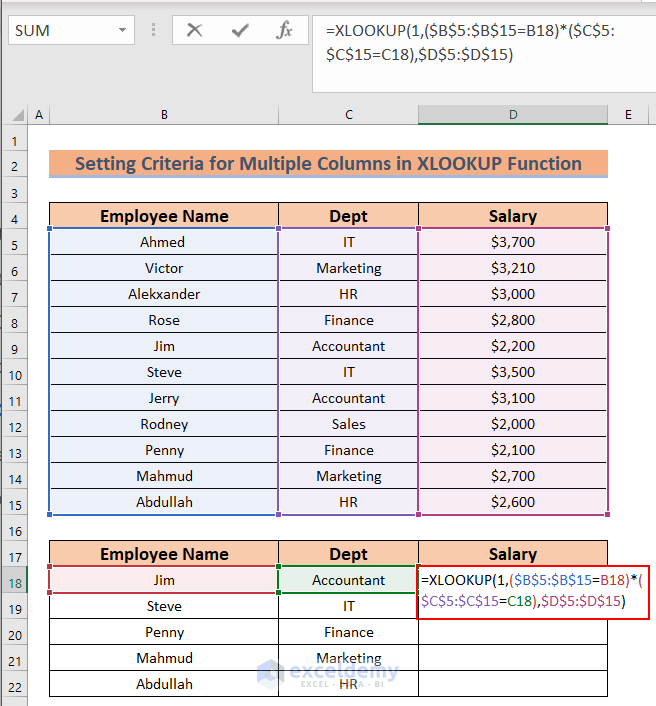
Case 1.2 – Set Criteria for Multiple Columns Separately
Steps:
- Select the cell where you want to place your resultant value. We selected cell D18.
- Insert the following formula in the selected cell or into the Formula Bar.
=XLOOKUP(1,($B$5:$B$15=B18)*($C$5:$C$15=C18),$D$5:$D$15)
Formula Breakdown
- We look up the Salary of Jim who works at Accountant department.
- The lookup_value is 1.
- We selected the lookup_array B5:B15=B18 * C5:C15=C18.
- We selected the return_array D5:D15.
- Press the Enter key.
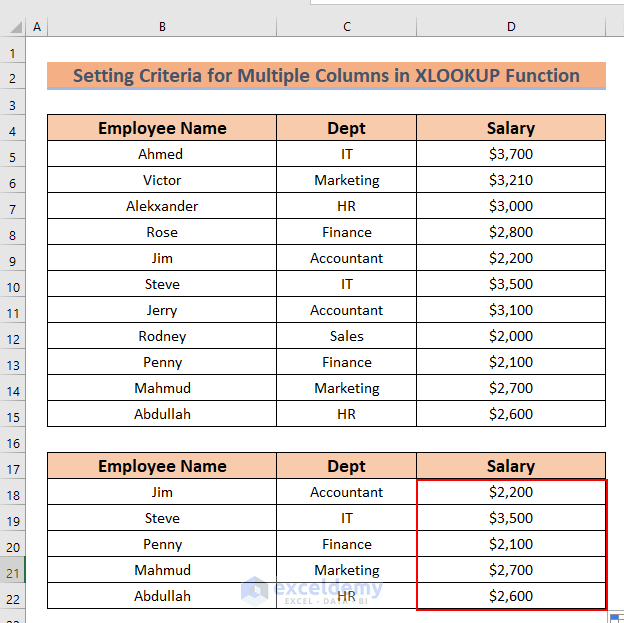
- Use the Fill Handle to AutoFill formula for the rest of the cells of the Salary column.
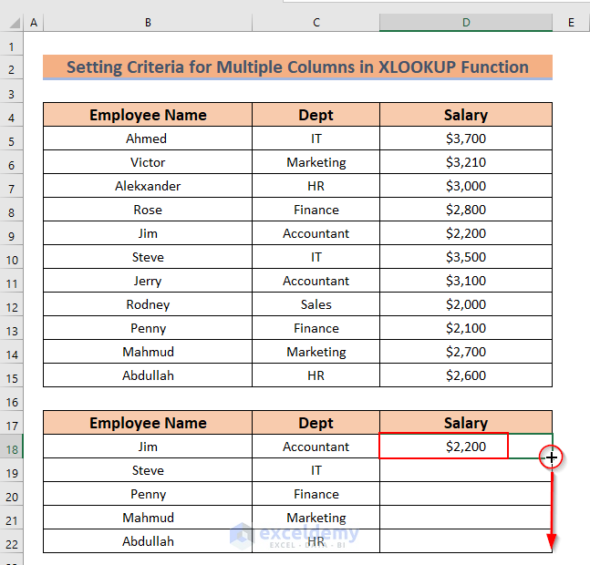
- You can see the complete Salary column.
Read More: VLOOKUP with Multiple Criteria Including Date Range in Excel
Method 2 – Combining Two XLOOKUP Functions for Multiple Criteria in Excel
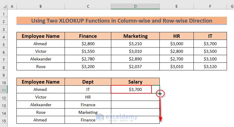
Case 2.1 – Using XLOOKUP Function Row-Wise then Column-Wise
Steps:
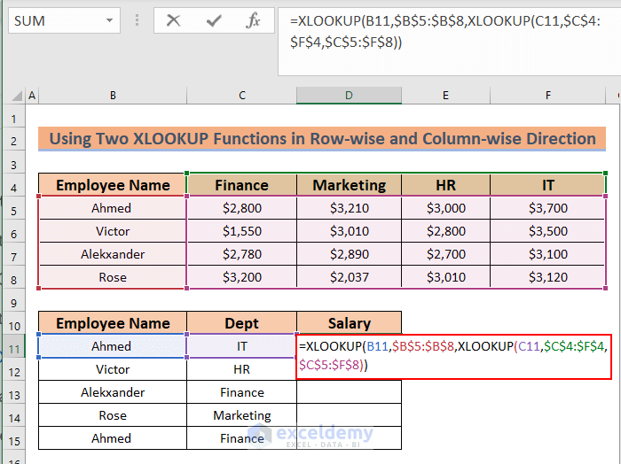
- Select the cell to place your resultant value. We selected cell D11.
- Insert the following formula in the selected cell or into the Formula Bar.
=XLOOKUP(B11,$B$5:$B$8,XLOOKUP(C11,$C$4:$F$4,$C$5:$F$8))
Formula Breakdown
- We want to look up the Salary of Ahmed who works in IT.
- We have the lookup_value B11 and selected the lookup_array as B5:B8.
- The outer XLOOKUP function searches column-wise.
- We used the XLOOKUP function and selected the 2nd criterion C11.
- The inner XLOOKUP function searches row-wise.
- The lookup_array is C4:F4 with the return_array C4:F8.
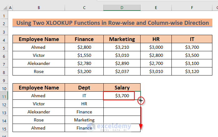
- Hit Enter.
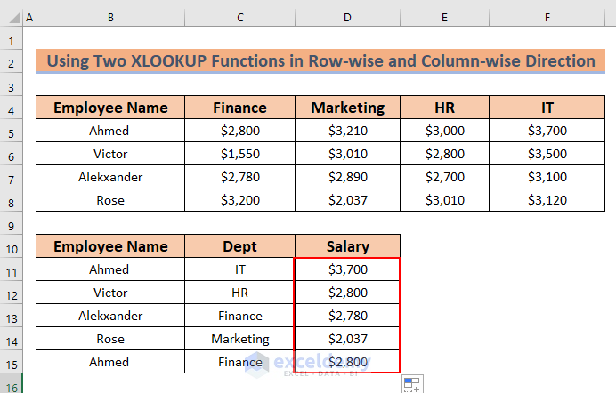
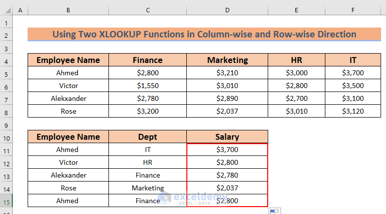
- Use the Fill Handle to AutoFill formula for the rest of the cells in Salary.
- You can see the complete Salary column.
Case 2.2 – Applying the XLOOKUP Function Column-Wise then Row-Wise
Steps:
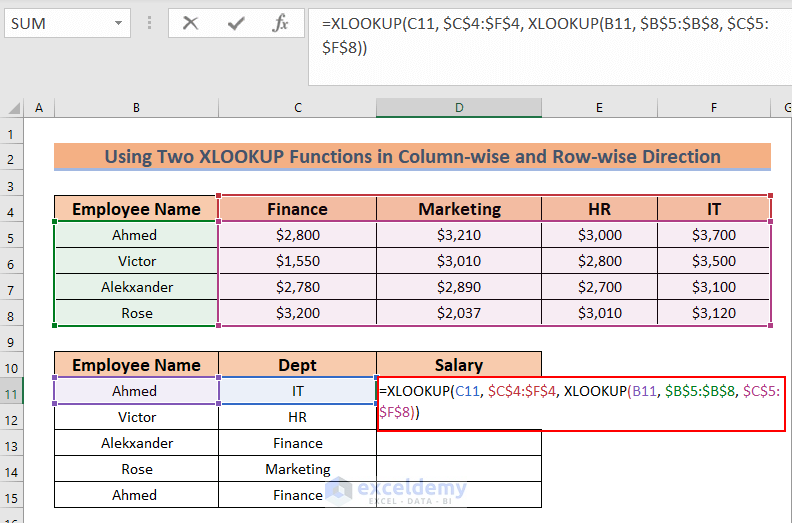
- Select the cell to place your resultant value. We selected cell D11.
- Insert the following formula in the selected cell or into the Formula Bar.
=XLOOKUP(C11, $C$4:$F$4, XLOOKUP(B11, $B$5:$B$8, $C$5:$F$8))
Formula Breakdown
- We just interchanged the lookup values from the inner to outer XLOOKUP function from the previous case.
- Hit Enter.
- Drag down the formula with the Fill Handle tool.
- You can see the complete Salary column.
Read More: Vlookup with Multiple Criteria without a Helper Column in Excel
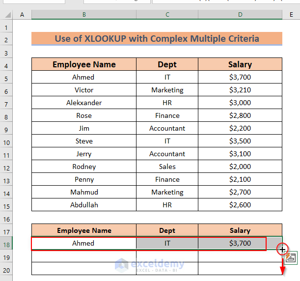
Method 3 – Applying the XLOOKUP Function with Advanced Multiple Criteria in Excel
Steps:
- Select the cell to place your resultant value. We selected cell B18.
- Insert the following formula in the selected cell or into the Formula Bar.
=XLOOKUP(1,(LEFT(B5:B15)=”A”)*(C5:C15=”IT”),B5:D15)

Formula Breakdown
- The LEFT function for the lookup_value “A” searches within the selected range B5:B15.
- For the 2nd criterion, we used the “=” with lookup_value inside the selected range C5:C15.
- We selected the range B5:D15 as return_array.
- Hit Enter.
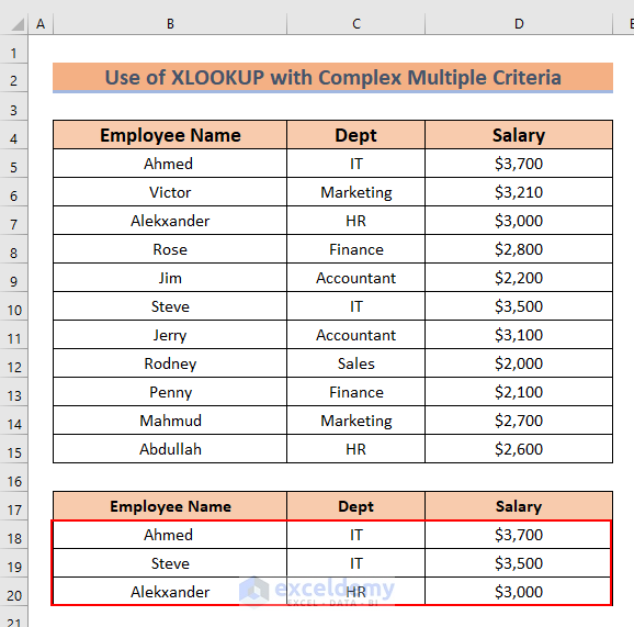
- Use the Fill Handle to AutoFill formula for the rest of the cells of the Salary column.
- You can see the result.
Read More: How to Lookup Across Multiple Sheets in Excel
Method 4 – Inserting a XLOOKUP Function with Multiple Logical Criteria in Excel
Steps:
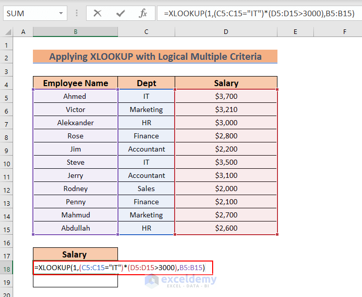
- Select the cell to place your resultant value. We selected cell F4.
- Insert the following formula in the selected cell or into the Formula Bar.
=XLOOKUP(1,(C5:C15="IT")*(D5:D15>3000),B5:B15)
Formula Breakdown
- We will use boolean logic to look for the number.
- In the XLOOKUP function we put the lookup_value “1” with the selected range C5:C15. For the second criterion, we used the “>” operator with lookup_value within the selected range D5:D15.
- We selected the range B5:B15 as return_array.
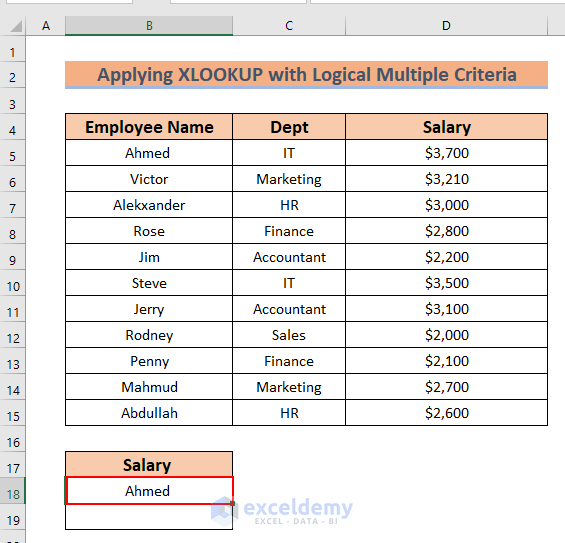
- Hit Enter.
- This will show the Salary of the given lookup_value.
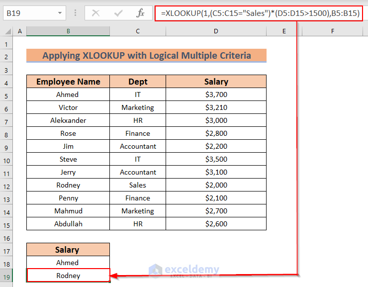
- Insert the following formula for cell B19.
=XLOOKUP(1,(C5:C15="Sales")*(D5:D15>1500),B5:B15)
- Hit Enter
- You can see the result in cell B19.
Read More: Lookup and Return Multiple Values Concatenated into One Cell in Excel
Download the Practice Workbook
Further Readings
- How to Use INDEX MATCH with Multiple Criteria for Date Range
- VBA INDEX MATCH Based on Multiple Criteria in Excel
- INDEX-MATCH with Multiple Criteria for Partial Text in Excel
- How to Use XLOOKUP to Return Blank Instead of 0


Hi Shamima,
Hope you r good, this article is so helpful in understanding xlookup function. Can you guide me actually i want to xlookup a value with a tolerance level of + & – in a lookup array. means i want to lookup a number & if it is found with + or – (tolerance) in a lookup up array it returns the result ..thanks you
Atif
Hello Atif Hassan,
Thanks for your appreciation. You can use the following formula to use XLOOKUP with tolerance level:
=XLOOKUP(TRUE, IF(ABS($C$2:$C$4 – $A$2) <= $B$2, TRUE, FALSE), $D$2:$D$4, "Not Found")
https://www.exceldemy.com/wp-content/uploads/2024/05/XLOOKUP-Based-on-Customized-Criteria.gif
Please download the Excel file for better understanding:
XLOOKUP with Tolerance Level.xlsx
Regards
ExcelDemy