How to Vlookup from Excel to Google Sheets (3 Suitable Ways)

Nowadays, Google Sheets is very convenient and suitable for syncing and working together simultaneously. For various purposes, you may need to extract data from Excel to Google Sheets. To do this, we’ve to upload the Excel file to Google Drive first or have to import the Excel file to Sheets directly. In this article, we’ll demonstrate 3 easy methods to use the VLOOKUP function to get data from Excel to Google Sheets. So, let’s go through it completely to apply them in your work too.

Vlookup from Excel to Google Sheets: 3 Suitable Methods

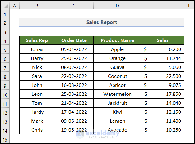
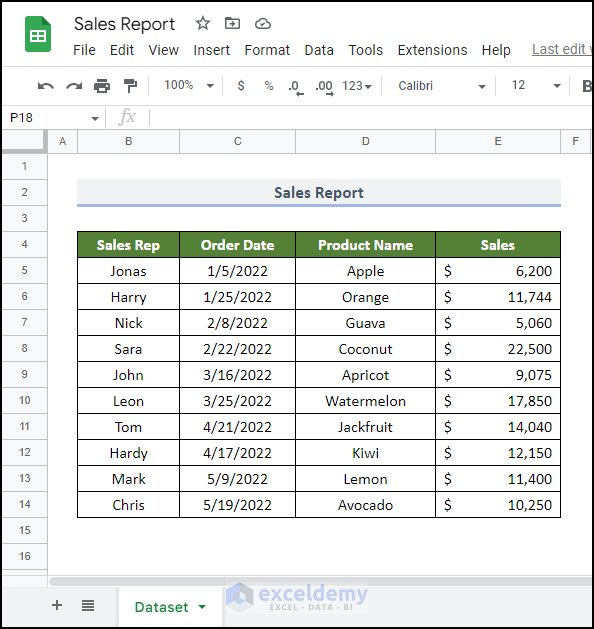
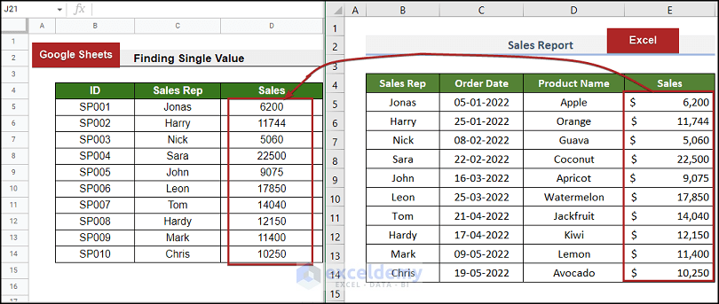
For ease of understanding, we are going to use a Sales Report of a particular grocery store. This dataset concludes the Sales Rep, Order Date, Product Name, and the corresponding Sales amount in columns B, C, D, and E respectively.

Now, we’ll apply the VLOOKUP function using 3 different approaches to fetch data from this Excel workbook to Google Sheets. So, let’s explore them one by one.
Here, we have used Microsoft Excel 365 version, you may use any other version according to your convenience.

1. Find Single Value

First of all, we’ll use the VLOOKUP function to find a single value. That means each formula will fetch just one value at a time. Without further ado, let’s see the method step-by-step.

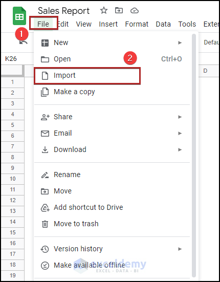
Step 01: Import Excel File to Sheets

At the very beginning, we should import our Excel (.xlsx) file to Google Sheets for further use. To do this,

• At first, create a blank spreadsheet in Sheets.
• Then, go to the File tab.
• After that, select Import from the list.

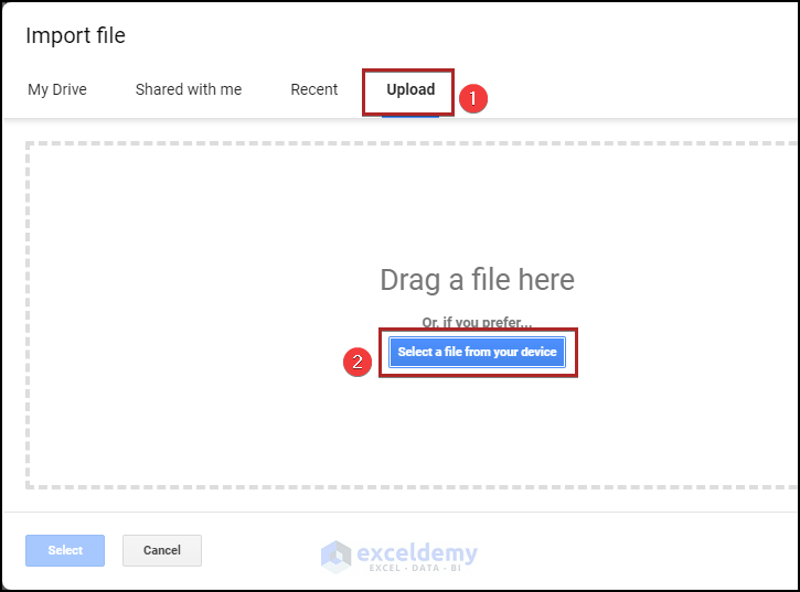
Immediately, the Import file dialog box appears.

• Here, move to the Upload tab.
• Afterward, click on Select a file from your device.

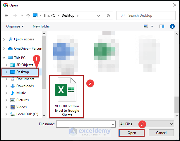
The Open window has now appeared in front of us.

• Currently, select Desktop where we kept the file. You can take id as your need.
• After that, select the desired file.
• Consequently, click on the Open button.

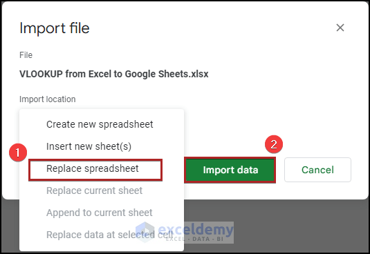
One more time, the Import file dialog box pops up.

• Presently, select Replace spreadsheet as the Import location.
• Henceforth, click on the Import data button.

Finally, the dataset is available on our Sales Report Google Sheets spreadsheet.

You can notice that the sheet name is also the same as in the Excel workbook, which is “Dataset”.

Step 02: Insert Formula

In the second step, we’ll do our main work. We’ll construct the formula using the VLOOKUP, and IMPORTRANGE functions of Google Sheets. So. let’s see it in action.

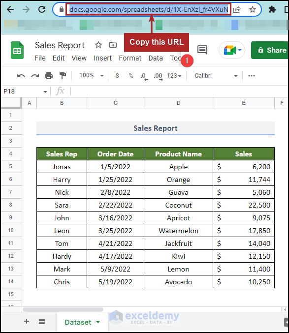
• Before going any further, copy the URL of the Sales Report sheet.

• Then, move to the new sheet named VLOOKUP from Excel to Google Sheet. Here, we can see the columns of ID and names of the Sales Rep are already present. We just have to extract the corresponding Sales amount for each Sales Rep.
• Firstly, select cell D5 and enter the following formula.

In this formula, C5 is the cell reference for Jonas. Because we want the number of his sales. Here, the part inside the double quotes of the IMPORTRANGE function is the URL of the Sales Report sheet. This function helps to import data from another Google Sheet. 4 is the index of the VLOOKUP function as the Sales column is in the 4th position of the table in the Sales Report sheet. And we used FALSE as the dataset is not sorted.

• Later, press ENTER.

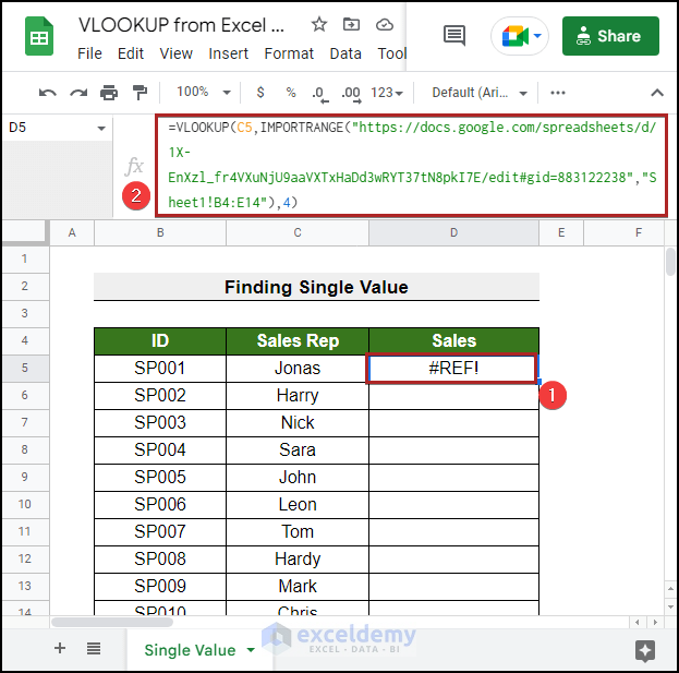
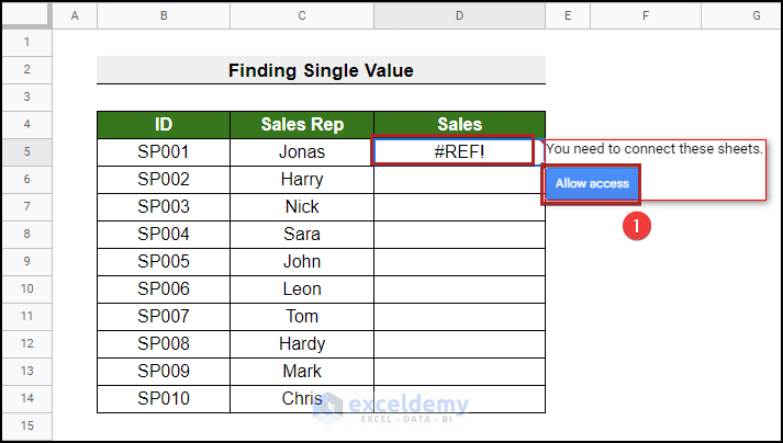
But we cannot see the proper results in cell D5. Rather, it shows a #REF error to us. Why is this happening? Don’t be tense.

• Again, click on cell D5.
• Instantly, it will show an error notification that You need to connect these sheets. And for this, we’ve to give access to the sheet.
• Next, click on Allow access in the message box.

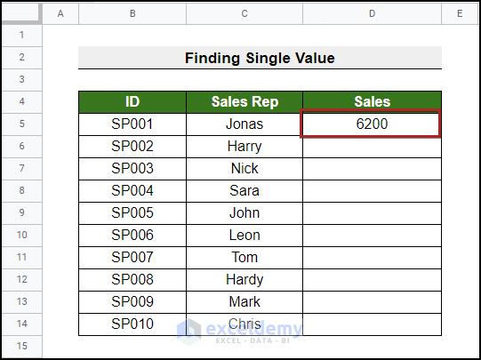
At this time, we can clearly see the output in that cell, which is 6200.

So, here, this formula returns a single value at a time. We can find the Sales amount of the remaining persons just by changing the search_key argument. For example, to find the Sales amount for Tom, use C11 instead of C5 in the same formula.

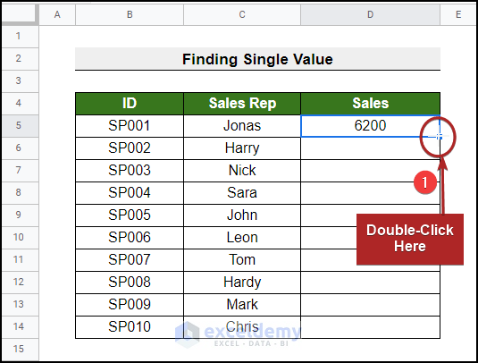
• Now, bring the cursor to the right-bottom corner of cell D5 and it’ll look like a plus (+) sign. Actually, it’s the Fill Handle tool.
• Hence, double-click on it.

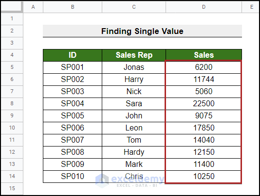
All the remaining cells get their outputs as the Fill Handle tool copies the same formula to the following cells also.

Step 03: Compare Excel File to Sheets

Now, we’ll compare the two files side by side to verify if the formula is correct. Let’s see the image below.
The right one is the Excel file, and the left one is the Google Sheet.

Read More: How to Save Excel Files to Google Sheets

2. Fetch Multiple Values in the Same Column

In our second method, we will repeat the previous method but change the formula slightly to produce an array output. So, without further delay, let’s dive in.

📌 Steps:

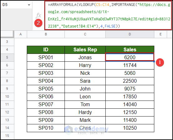
• Firstly, go to cell D5 and insert the formula below.

Here, the VLOOKUP function will return the lookup value of all the sales reps in the C5:C14 range. For this, we’ve added the ARRAYFORMULA function to get an array output.

• Secondly, tap ENTER.

Using this formula, we were able to get all of the Sales at once. There is no need to use the Fill Handle in this case.

3. Apply VLOOKUP Function with Wildcard or Inadequate Matches

In the third and last method, we’ll learn to use a wildcard or partial match to apply VLOOKUP in the Google Sheets file. So, let’s begin.

📌 Steps:

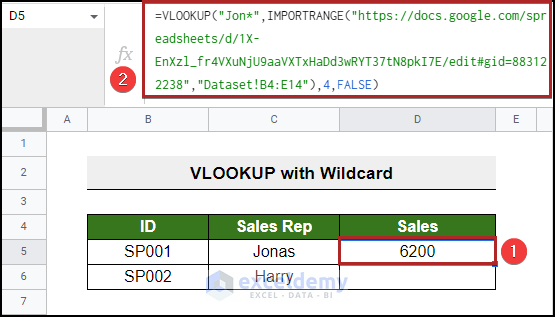
• Primarily, select cell D5 and paste the following formula into the cell.

Here, we’ve used “Jon*” as the search_key. So, the function will search for text strings containing these texts and will return the Sales amount.

• Secondarily, hit the ENTER key.

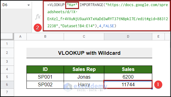
To extract the sales from Harry, edit the formula a little bit.

• Next, write down “Ha*” instead of “Jon*”.
• Also, press ENTER.

Things to Remember

Before using the IMPORTRANGE function, make sure to change the privacy of the sheet from Restricted to Anyone with the link. Otherwise, it will return the #REF error.

Download Practice Workbook

You may download the following Excel workbook for better understanding and practice yourself.

Conclusion

This article explains how to use the VLOOKUP function to import data from Excel to Google Sheets in a simple and concise manner. Don’t forget to download the Practice file. Thank you for reading this article. We hope this was helpful. Please let us know in the comment section if you have any queries or suggestions.