So,This tutorial will demonstrate how to use VLOOKUP and HLOOKUP Combined formulas together in Excel formulas. Moreover, we can find specific data or formulas or groups of formulas or data by using these functions. If you use these functions, it will search the particular data you have inserted. In case, you want to find a certain column or group of columns in the worksheet, then naming the table array is very useful. After naming a table array, you can find it with selected cells under it only by searching by the proper name. So, it shortens our work and is essential for us to learn using it quickly.
Download Practice Workbook
You can download the practice workbook from here.
Overview of VLOOKUP Function
- Description
In case, if you are looking up a value vertically in Excel, you need to use the VLOOKUP function. Undoubtedly, it is a very useful built-in function in Excel that is under the Lookup function category. VLOOKUP Function is mainly used when you have to find a table or some info or any data by row.
- Generic Syntax
=VLOOKUP (Lookup_Value, Table_Range, Column_Index, [Range_Lookup])
- Argument Description
Arguments | Requirements | Explanation |
---|---|---|
Lookup_Value | Required | The value which you will look up vertically from the first column of the Table_Range. |
Table_Range | Required | Defines the range of the VLOOKUP function. |
Column_Index | Required | The column number from the Table_Range by which the matched value will be returned. |
Range_Lookup | Optional | It’s an optional argument. Write False to get Exact Match and True for an approximate match. True is the default parameter while omitting this argument. |
Example:
Overview of HLOOKUP Function
- Description
If you want to look up a value horizontally in Excel you need to use the HLOOKUP function. It is also a built-in function in Excel which is under the Lookup function category. Moreover, the HLOOKUP or Horizontal Lookup function is generally used to extract data from a table or an array based on searching for a specified value in the topmost row and the corresponding column.
- Generic Syntax
=HLOOKUP (Lookup_Value, Table_Range, Row_Index, [Range_Lookup])
- Argument Description
Arguments | Requirements | Explanation |
---|---|---|
Lookup_Value | Required | The value which you will look up vertically from the first column of the Table_Range. |
Table_Range | Required | Defines the range of the HLOOKUP function. |
Row_Index | Required | The row number from the Table_Range by which the matched value will be returned. |
Range_Lookup | Optional | It’s an optional argument. Write False to get Exact Match and True for an approximate match. True is the default parameter while omitting this argument. |
Example:
Step-by-Step Procedures to Use VLOOKUP & HLOOKUP Combined Formula Together in Excel
If you follow the steps correctly, you should learn how to use both VLOOKUP and HLOOKUP combined formulas together in excel to ease the work. So, we have to follow the below steps to learn this method.
Steps:
- First, arrange the proper dataset that you want to use. Now, we have the Salesperson in Column B and two years 2021 and 2022 in Column C and D.
- Next, in cell D14 insert the following formula.
=VLOOKUP(B14,B5:D11,2,0)
- After that, you will get the desired result.
🔎 How Does the Formula Work?
How to Use IF Statement with VLOOKUP Function
We will learn how to combine the IF, VLOOKUPÂ & HLOOKUPÂ functions. The If function gives logical comparison, and VLOOKUPÂ & HLOOKUPÂ functions find specific data from a certain range. The process to learn this method are.
1. IF Statement with VLOOKUP Function
We can ease our work by combining the IF statement with the VLOOKUP function. So, we have to follow the following steps to learn this whole process.
Steps:
- Now, in cell D14 insert the following formula.
=IF(VLOOKUP(B14,$B$4:$D$11,3,FALSE )>=30000, VLOOKUP(B14,$B$4:$D$11,3,FALSE)*20%, VLOOKUP(B14,$B$4:$D$11,3,FALSE)*10%)
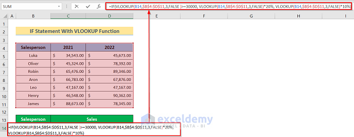
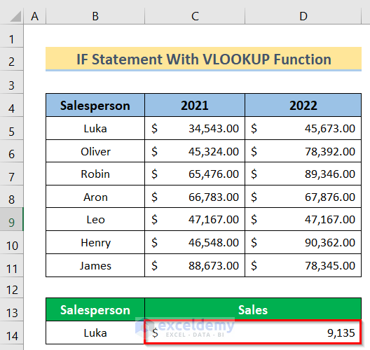
- Finally, you will get the desired result.
🔎 How Does the Formula Work?
Read More: How to Find Duplicate Values Using VLOOKUP in Excel
2. IF Statement with HLOOKUP Function
We can also do the same work by combining the IF statement with the HLOOKUP function. Now, for doing so we have to follow the following steps.
Steps:
- Next, in cell B14 insert the following formula.
=HLOOKUP(B13,B4:D11,IF(D10>30000,7))
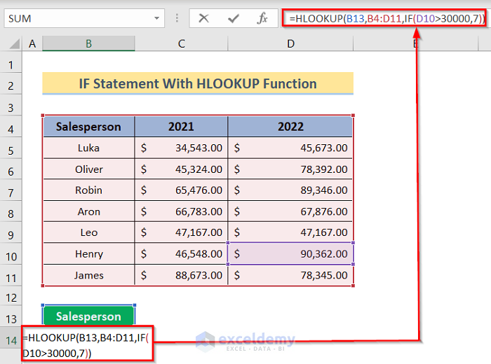
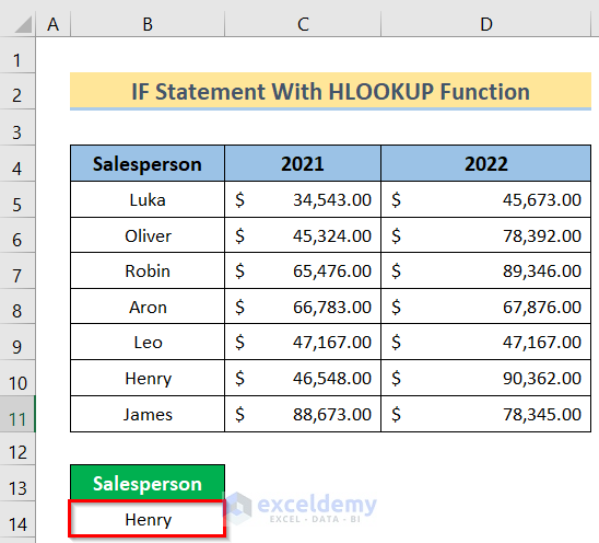
- Finally, you will get the desired result.
🔎 How Does the Formula Work?
Conclusion
Henceforth, follow the above-described methods. Thus, you will be able to learn the basics of the VLOOKUP and HLOOKUP combined formulas. So, let us know if you have more ways to do the task. Follow the ExcelDemy website for more articles like this. Don’t forget to drop comments, suggestions, or queries if you have any in the comment section below.
Great instruction on how to use both VLOOKUP and HLOOKUP functions! I like this.
Thanks for your feedback, George!
its very good example
Thanks for your feedback.
I’d love to have a few exercises to apply this knowledge in order to assimilate it properly. Thanks for considering this request.
Hi,
You can try to use the concepts in real-world problems.
Thanks.
I can’t believe I just understood this…Appreciate the clear example, you are a great instructor!
Hi Kawser.. thanks for the blog post on doing a 2-way lookup using VLOOKUP and HLOOKUP together. The weakness is that you have to convert the month reference to a number with a helper table. As you mentioned in your conclusion, a more direct approach would be to combine INDEX and MATCH for a 2-way lookup as follows (using your data set as example):
=INDEX($B$2:$E$9,MATCH($H$4,$A$2:$A$9,0),MATCH($H$5,$B$1:$E$1,0))
In this approach, no helper table is required to generate the month number for the column. The MATCH function does it for you. So, arguably it is more efficient. Either way works.. nice to know multiple methods to solve a problem. Thanks for your insights!
Thank you so much for your input, Wayne! Hope this input helps my readers 🙂
Best regards
Kawser Ahmed
Thanks for the well written and very helpful article by explaining the concepts clearly with examples.
hello sir i am microsoft certified trainer from Gujarat India, i am using your method and some example to explain formula during my lecture , thanks for your blog , lots of thanks – rajesh bhonkiya
A great pleasure for me. Thank you.
Hi Kawser, I have always enjoyed your blog posts, they are insightful and helpful. I have figured an alternative to Wayne’s suggestion – that would be to use a combination of vlookup and match: =VLOOKUP(H4,A1:E9,MATCH(H5,B1:E1,0)+1,0), without using an additional match.
This uses the match to return the column number of the selected month and subsequently vlookup to the product name based on the column number to obtain the product name for the given month.
Thanks to your blog posts, I have developed a strong interest in writing and understanding excel formulas.
Cheers!