How to Tabulate Data in Excel (4 Methods)

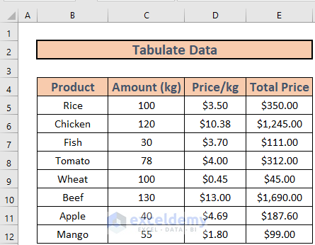
The sample dataset has some products, along with their price per unit (kg) and the amounts.

Method 1 – Use Insert Tab Option to Tabulate Data in Excel

Steps:

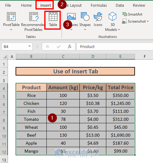
• Select the entire range B4:E12.
• Go to the Insert tab >> select Table.

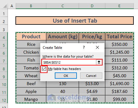
• Create Table box will pop up.
• Select the data range you want to tabulate.
• Check the My table has headers box if you want headers in your table.
• Click OK.

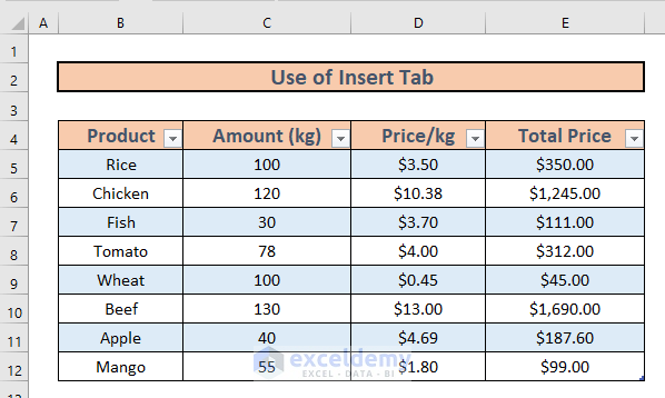
• Excel will tabulate your data.

Method 2 – Apply Keyboard Shortcut to Tabulate Data in Excel

Steps:

• Select any cell from your dataset.
• Press CTRL + T.
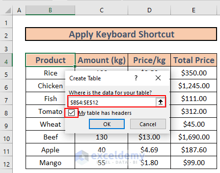
• The Create Table box appears.
• Select B4:E12 as the data range.
• Check the My table has headers box if you want headers in your table.
• Click OK.

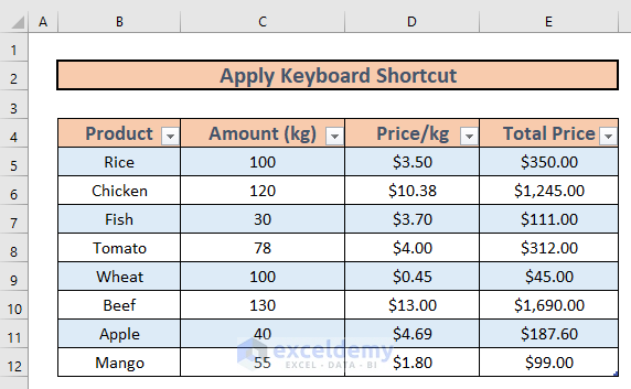
• Excel will tabulate your data.

Method 3 – Create Pivot Table to Perform Data Tabulation in Excel

Steps:

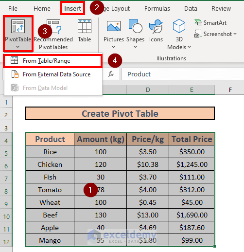
• Select B4:E12.
• Go to the Insert tab >> select Pivot Table >> select From Table/Range.

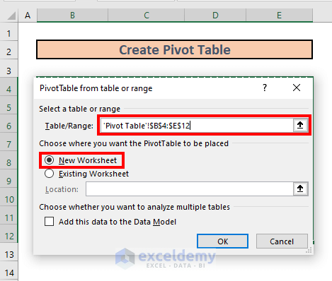
• A window will appear. Select your range.
• Choose the destination of your pivot table. New Worksheet has been selected as the destination in this instance.
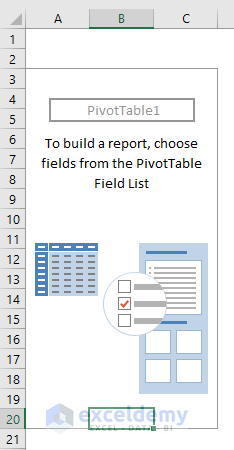
• Click OK.

• Excel will create a pivot table.

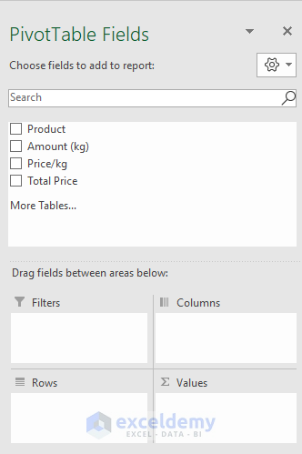
• From the PivotTable Fields, the data can be modified further.

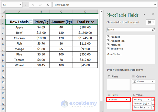
• For example, if Product is in the Rows and Amounts (kg), Price/kg, and Total Price are in the Values field, the pivot table will look like this.

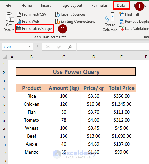
Method 4 – Use Power Query to Tabulate Data in Excel

Steps:

• Go to the Data tab >> select From Table/Range.

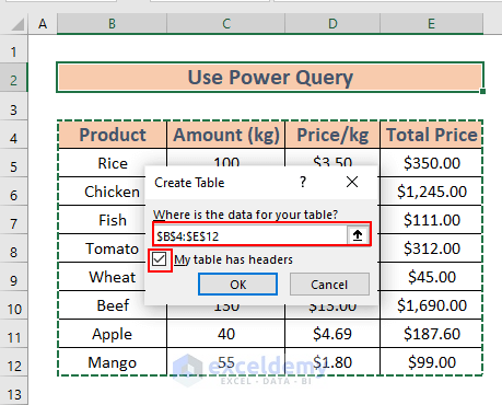
• Create Table box will pop up.
• Select the dataset and check the My table has headers box if you want headers in your table.
• Click OK.

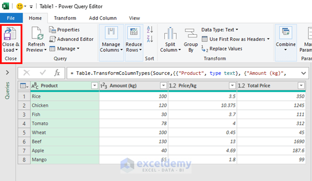
• Power Query Editor will appear. Click Close & Load.

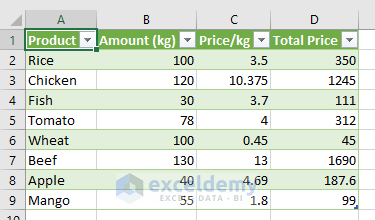
• Excel will create the data tabulation in another worksheet.

Read More: How to Analyze Satisfaction Survey Data in Excel

Things to Remember

• You can also create a pivot table by pressing ALT+N+V+T. Just remember that you have to press them one by one, not simultaneously.
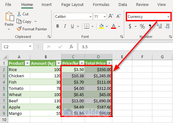
• Do not forget to change the format to Currency in the new table created by using Power Query.

Download Practice Workbook

Download this workbook and practice while going through this article.

Related Articles

• How to Tally Survey Results in Excel
• How to Display Survey Results in Excel
• How to Encode Survey Data in Excel
• How to Create a Questionnaire in Excel
• How to Analyze Survey Data with Multiple Responses in Excel
• How to Analyze Survey Data in Excel

<< Go Back to Survey in Excel | Excel for Statistics | Learn Excel