Looking for ways to know how to select specific rows in the Excel formula? Sometimes, we want to select specific rows in Excel that contain formulas or using formulas. Here, you will find 4 ways to select specific rows in the Excel formula.
How to Select Specific Rows in Excel Formula: 4 Ways
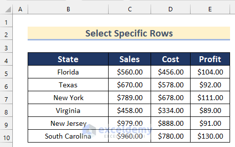
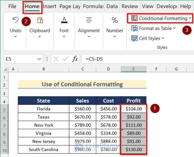
Here, we have a dataset containing the information about State, Sales, Cost, and Profit of a company. Now, we will use this dataset to show you how to select specific rows in Excel formula.
1. Using Keyboard Shortcut to Select Specific Rows in Excel Formula
In the first method, we will show you how to use Keyboard Shortcut to select specific rows in Excel based on formulas. Follow the steps given below to do it on your own.
Steps:
- Firstly, select Cell range E5:E10.
- Then, press CTRL+SHIFT+\.

- Now, you will see that the Cells that contain different formulas in the Cell range have been highlighted in your dataset. Here, in our dataset, Cell E8 and Cell E10 have been highlighted.

- Next, click on Bold to bold the Cell values.

- Afterward, click on Row 8.
- Next, press CTRL and then click on Row 10.
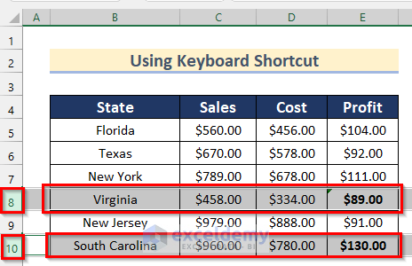
- After that, click on Bold to bold the data of Row 8 and Row 10.

- Thus, you can select specific rows in Excel using Keyboard Shortcut.

Read More: How to Select All Rows in Excel
2. Applying Find & Select Feature to Select Specific Rows
We can also select specific rows in Excel based on formulas by applying the Find & Select Feature. Go through the steps given below to do it on your own dataset.
Steps:
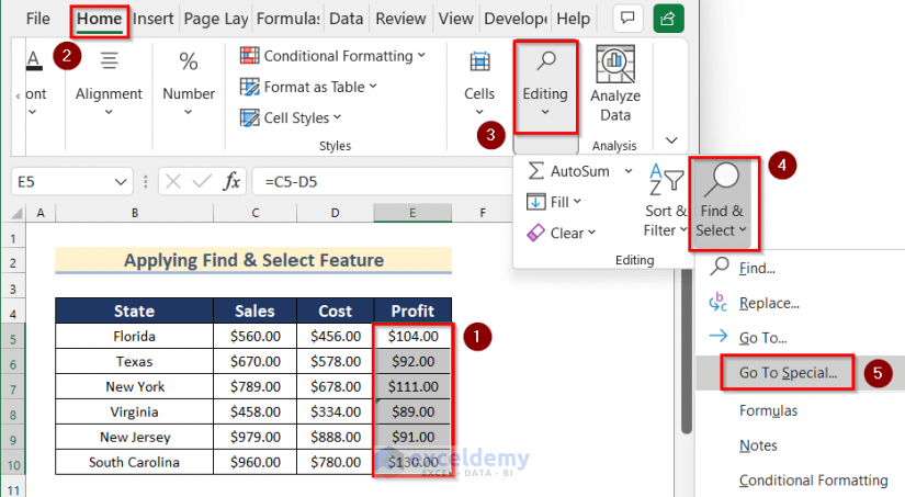
- In the beginning, select Cell range E5:E10.
- After that, go to the Home tab >> click on Editing >> click on Find & Select >> select Go to Special.
- Now, the Go to Special box will open.
- Then, select Column differences.
- Next, click on OK.

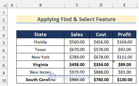
- Now, you will see that the Cells that contain different formulas in the Cell range have been highlighted in your dataset. Here, in our dataset, Cell E8 and Cell E10 have been highlighted.

- After that, click on Bold to bold the Cell values.

- Then, click on Row 8.
- Next, press CTRL and then click on Row 10.

- After that, click on Bold to bold the data of Row 8 and Row 10.

- Thus, you can select specific rows in Excel by applying the Find & Select Feature.
3. Use of Conditional Formatting to Select Specific Rows in Excel Formula
Now, we will show you how to use Conditional Formatting with formulas to select specific rows in Excel. Follow the steps given below to do it on your own.
Steps:
- Firstly, select Cell range E5:E10.
- Then, go to the Home tab >> click on Conditional Formatting.
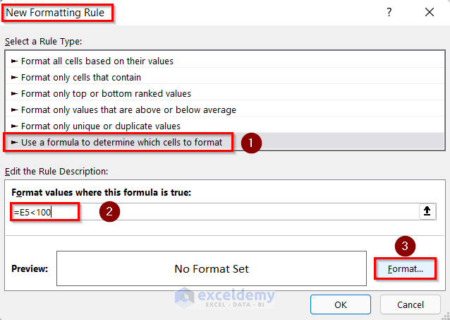
- Next, click on New Rule.

- Now, the New formatting Rule box will open.
- After that, select Use a formula to determine which cells to format.
- Then, insert the following formula in the box.
=E5<100Here, at first, we checked if Cell E5 is less than 100 or not.
- Next, click on Format.
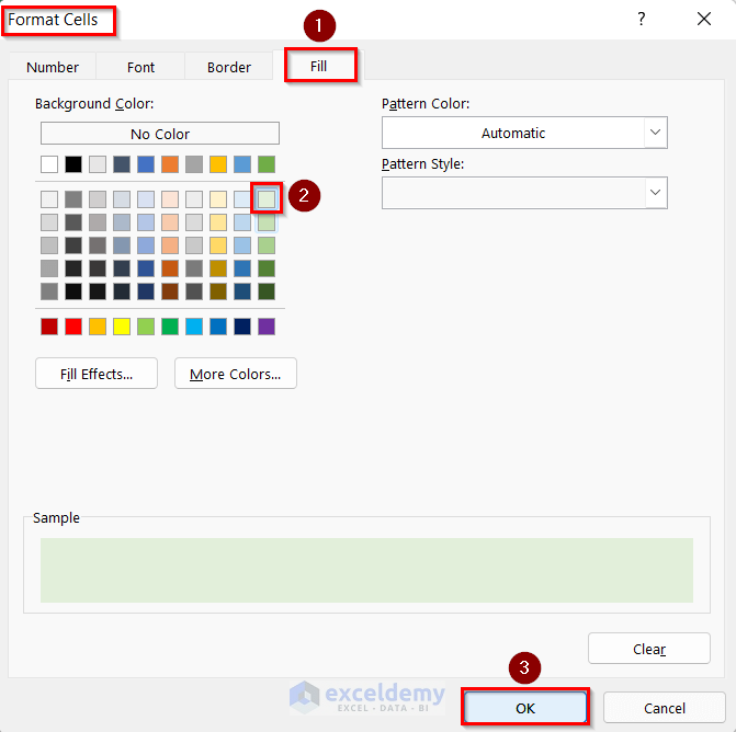
- Now, the Format Cells box will open.
- Afterward, go to the Fill option.
- Then, select any Background Color of your choice. Here, we will select Green, Accent 6, Lighter 80%.
- Next, click on OK.
- Again, the New Formatting Rule box will appear.
- After that, click on OK.

- Then, you will see that the Cell E6, Cell E8, Cell E9 are formatted according to the formula used in Conditional Formatting as the values less than 100.

- Afterward, click on Row 6.
- Next, press CTRL and then click on Row 8 and Row 9 .

- After that, click on Bold to bold data of Row 6, Row 8, and Row 9.

- Thus, you can select specific rows in Excel using Conditional Formatting.

4. Using Name Box to Select Specific Rows in Excel Formula
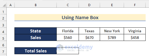
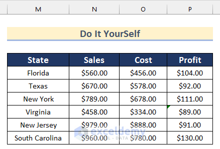
In the final method, we will show you how to use the Name Box to select specific rows in Excel. Here, we have a dataset containing the information about Sales in different States of a company. Now, we will show you how you can select a specific row using Name Box and use it in a formula.
Go through the steps given below to do it on your own dataset.
Steps:
- In the beginning, select Cell range B4:F5.
- Then, go to the Formulas tab >> click on Defined Names >> select Create from Selection.

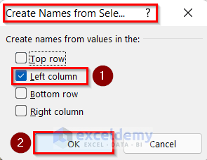
- Now, the Create Names from Selection box will open.
- After that, select the Left column option.
- Then, click on OK.
- Next, select Cell C7.
- Afterward, insert the following formula.
=SUM(Sales)
Here, in the SUM function, we inserted Sales which contains the values of Cell range C5:F5.
- Then, press ENTER.
- Thus, you can use Name Box to select specific rows in Excel

Read More: How to Select Every Other Row in Excel
Practice Section
In this section, we are giving you the dataset to practice on your own and learn to use these methods.
Download Practice Workbook
Conclusion
So, in this article, you will find 4 ways to select specific rows in Excel formula. Use any of these ways to accomplish the result in this regard. Hope you find this article helpful and informative. Feel free to comment if something seems difficult to understand. Let us know any other approaches which we might have missed here. Thank you!
Related Articles
- How to Select all Rows to Below in Excel
- How to Select Row in Excel If Cell Contains Specific Data
- How Do I Quickly Select Thousands of Rows in Excel
<< Go Back to Select Row | Rows in Excel | Learn Excel
Get FREE Advanced Excel Exercises with Solutions!
