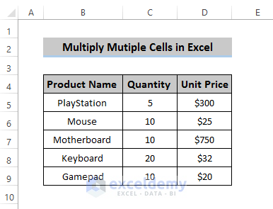
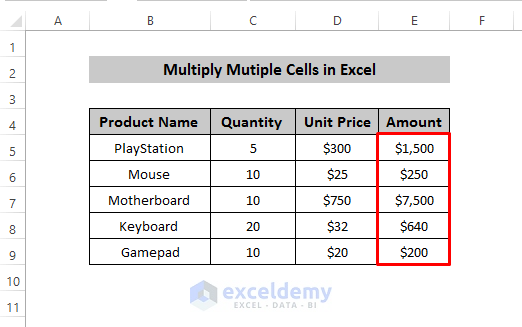
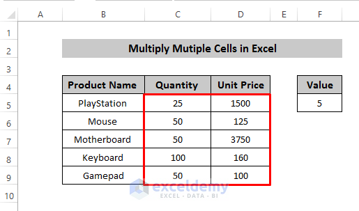
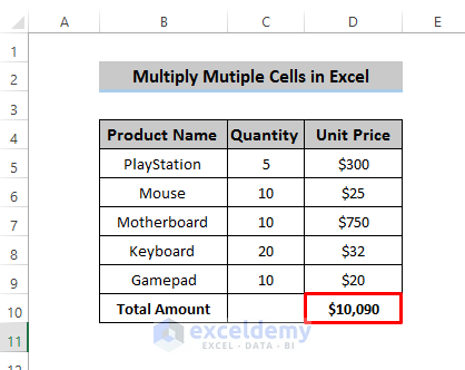
The sample dataset showcases product quantity and unit price.
Method 1 – Using the Asterisk Sign to Multiply Multiple Cells in Excel
Steps
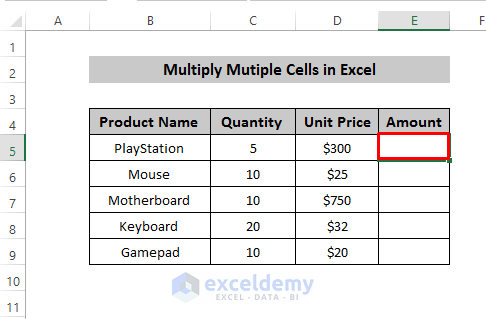
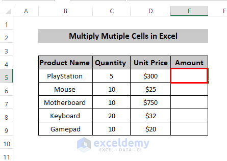
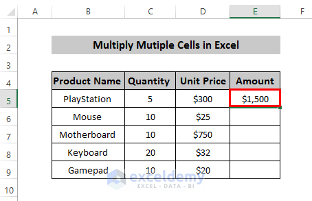
- Select a cell to display the value.
- In the formula bar, enter the equal sign (=). Supply your cell reference. Here, C5 is multiplied by D5. Enter the formula.
=C5*D5 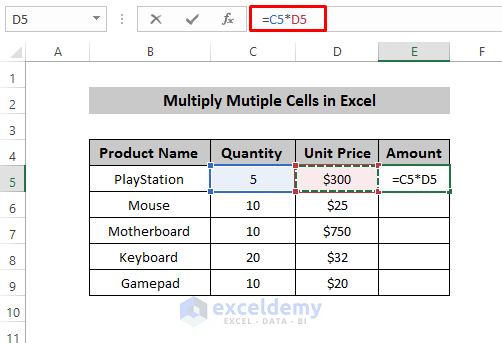
- Press Enter.
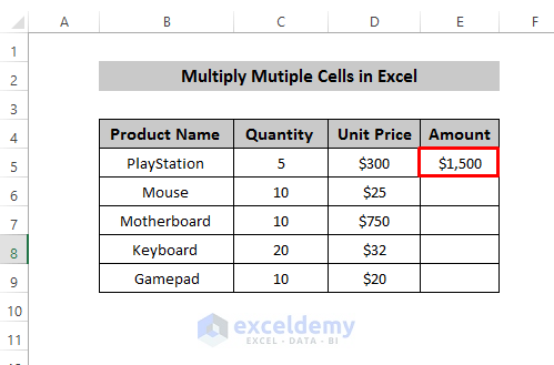
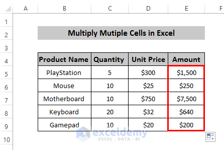
- Drag down the Fill Handle to apply the formula to the rest of the cells.
Read More: How to Multiply Two Columns in Excel
Method 2 – Applying the PRODUCT Function to Multiply Multiple Cells
Steps
- Select a cell to display the value.
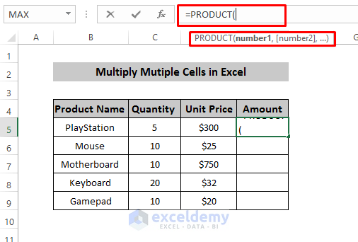
- Enter the equal sign (=) in the formula box.
- Enter Product.
- Enter number 1 (the first cell) and number 2 (the second cell). More numbers can be used separated by a comma.
- To multiply C5 by D5, enter the following function.
=PRODUCT(C5,D5)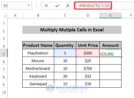
- Press Enter.
- Drag down the Fill Handle to apply the formula to the rest of the cells.
Read More: How to Create a Multiplication Formula in Excel
Method 3 – Multiplying Multiple Cells with a Constant Value in Excel
3.1 Using Paste Special Command
Steps
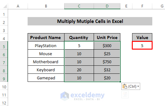
- Set a constant value in a blank cell. Here, ‘5’ .
- Copy it and select the range of cells you want to multiple by the constant value.
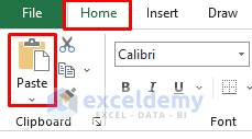
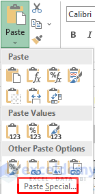
- Go to the Home tab and click Paste.
- In Paste, select Paste Special.
- In the Paste Special dialog box, select All in Paste, and Multiply in Operation.
- Click ‘OK’.

This is the output.
3.2 Applying a Formula in Excel
Steps
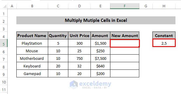
- Enter a constant value in a blank cell.
- Select a column to display the result of the multiplication.
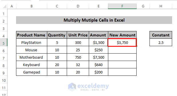
- Enter the Equal Sign (=). Select the cell reference and the constant value cell reference. Use the Asterisk Sign (*) between the two cell references. Enter the following formula:
=E5*$H$5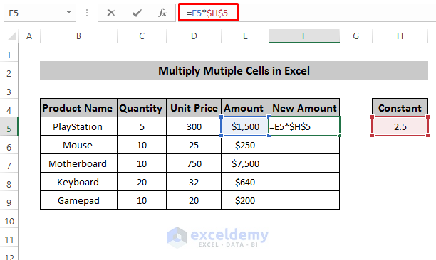
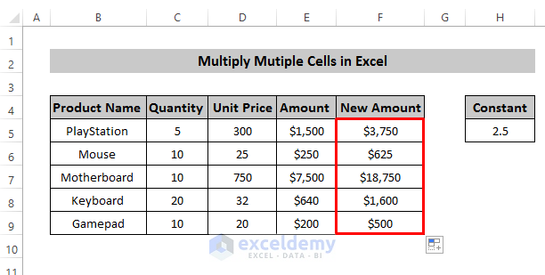
- Press Enter to see the result.
- Drag down the Fill Handle to apply the formula to the rest of the cells.
Note: Here, you can see we use a dollar sign ($) to represent the constant value cell reference. The dollar sign can transform the constant value reference into an absolute cell reference.
Read More: How to Multiply Rows in Excel
Method 4 – Creating an Excel Array Formula to Multiply Multiple Cells
Steps
- Select a cell to enter the Array formula.
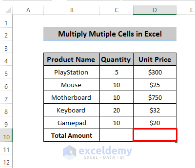
- Enter the Equal sign (= . Enter the following formula.
=SUM(C5:C9*D5:D9)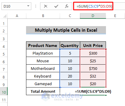
- Press Ctrl+Shift+Enter to apply the formula.
Things to Remember
For an array function press Ctrl+Shift+Enter to apply the formula.
Download Practice Workbook
Download the practice workbook.
Related Articles
- How to Do Matrix Multiplication in Excel
- How to Multiply from Different Sheets in Excel
- How to Multiply by Percentage in Excel
- How to Multiply Two Columns and Then Sum in Excel
- How to Divide and Multiply in One Excel Formula
- If Cell Contains Value Then Multiply Using Excel Formula
- How to Make Multiplication Table in Excel
<< Go Back to Multiply in Excel | Calculate in Excel | Learn Excel
Get FREE Advanced Excel Exercises with Solutions!
