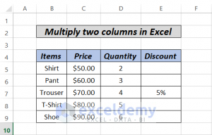
We’ll use a sample dataset as an example to help you understand how to multiply columns.
We are given Names of some Items in column B, Prices in column C, Quantities in column D, and Discount percentages in column E. We want to calculate the total Sales.
Method 1 – Using the Asterisk Symbol to Multiply Two Columns in Excel
Suppose we want to know how much Sales is generated for a particular product.
- Click on cell E5.
- Go to the formula bar and insert the following formula:
=C5*D5
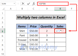
- Press Enter.
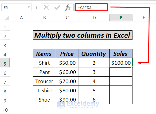 Here, we are multiplying two cells C5 with Cell D5 using the Asterisk (*) symbol. We got the result of $100 as the Sales value.
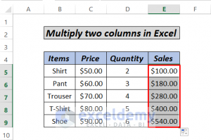
- Click on the bottom-right corner of the cell and drag it down. This is using the AutoFill feature to fill other cells automatically.
Read More: How to Multiply Multiple Cells in Excel
Method 2 – Multiplying Two Columns with the PRODUCT Formula
In our data set, we want Sales values by multiplying Price and Quantity.
- Insert the following formula in E5:
=PRODUCT(C5:D5)
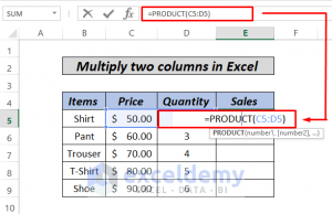
- Press the Enter key. It will show you the result.
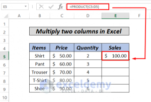
- We have the result of $100 as Sales value in cell E5. Excel is simply multiplying cells C5 and cell D5.
With the PRODUCT function, we can select desired cells using a colon (:) or comma (,). In this scenario, we can also use the formula as
=PRODUCT(C5,D5)
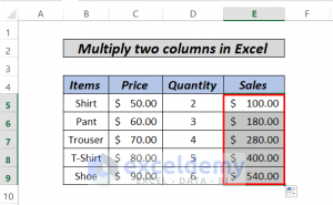
- Use AutoFill. Click the bottom-right corner of the cell and drag it down.
Read More: How to Create a Multiplication Formula in Excel
Method 3 – Multiplying Two Columns by a Constant Number
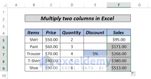
In our data set, we can see that there is a 5% Discount. We want to calculate sales value after the discount.
- Click on cell F5 and use the following formula.
=C5*D5*(1-$E$7)
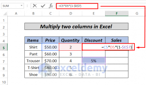
- Press the Enter key.
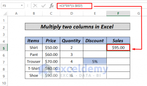
We are multiplying cells C5, D5, and E7. We also used the Absolute Reference for cell E7. Here, we subtracted the discount value to get the total Sales after the discount.
You use an Absolute Cell Reference (like $E$7) to ensure that the column and row coordinates of the cell containing the number to multiply by do not change while copying the formula to other cells.
You use a Relative Cell Reference (like C4) for the topmost cell in the column. When the formula is copied, this reference changes to the appropriate row and column. The formula in F6 changes to =C6*D6*(1-$E$7), the formula in F7 changes to =C7*D7*(1-$E$7), and so on.
- AutoFill to the other cells in the column.
Read More: How to Multiply by Percentage in Excel
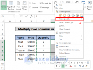
Method 4 – Using Excel Paste Special to Multiply Two Columns
- Copy values from columns D5 to D9 into columns E5 to E9.
- Select all the values in column C. We selected the range C5:C9.
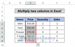
- Right-click and select Copy from the context menu.
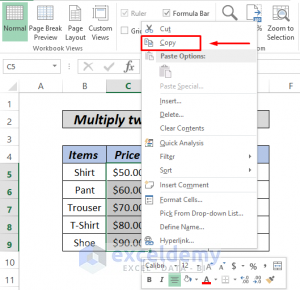
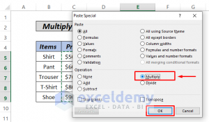
- Select cells E5:E9, then right-click.
- Select Multiply then click on OK.
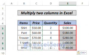
- You will get Sales for all the selected Items.
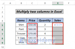
Method 5 – Multiplying Two Columns in Excel with an Array Formula
- Select cells from E5 to E9 (E5:E9).
- Type =C5:C9 or simply select all the required cells by dragging the mouse.
- Type the asterisk symbol and select cells D5:D9.
- The formula will be as given.
=C5:C9*D5:D9
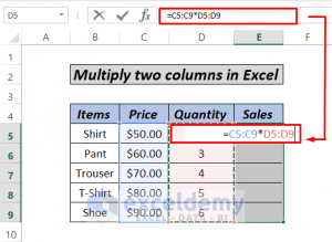
- Press Ctrl + Shift + Enter together as it’s an array formula.
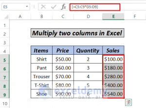
We multiplied C5 with D5, C6 with D6, and so on until C9 with D9.
Download the Practice Workbook
Related Articles
- How to Divide and Multiply in One Excel Formula
- How to Do Matrix Multiplication in Excel
- How to Multiply from Different Sheets in Excel
- How to Make Multiplication Table in Excel
- How to Multiply Rows in Excel
- How to Multiply Two Columns and Then Sum in Excel
- If Cell Contains Value Then Multiply Using Excel Formula
<< Go Back to Multiply in Excel | Calculate in Excel | Learn Excel
Get FREE Advanced Excel Exercises with Solutions!
