How to Do Matrix Multiplication in Excel (5 Examples)

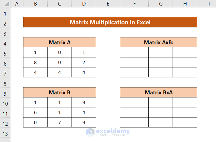
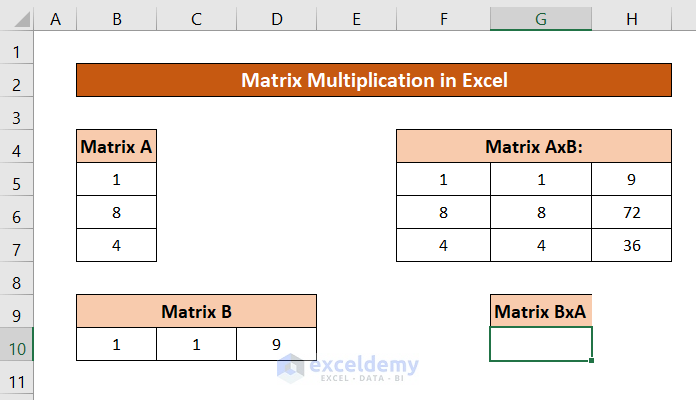
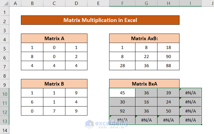
Method 1 – Performing Matrix Multiplication of Two Arrays in Excel

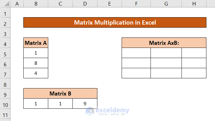
Let’s take two individual matrices A and B. In Excel, we will treat them as arrays for matrix multiplication.

Steps:

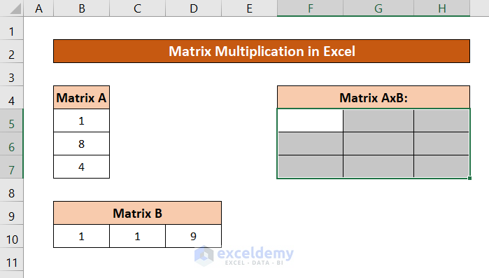
• Select the cells you want to put your matrix in.

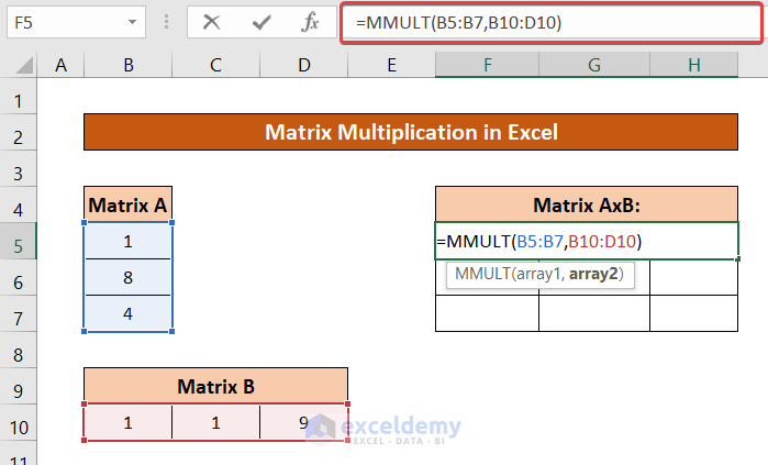
• Enter the following formula:

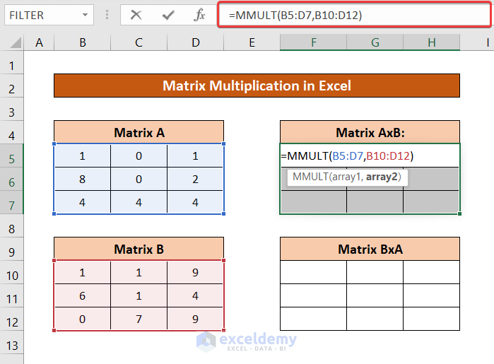
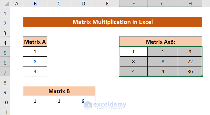
• Press Ctrl+Shift+Enter to get the result of the AxB matrix.

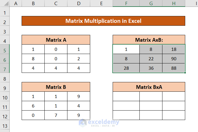
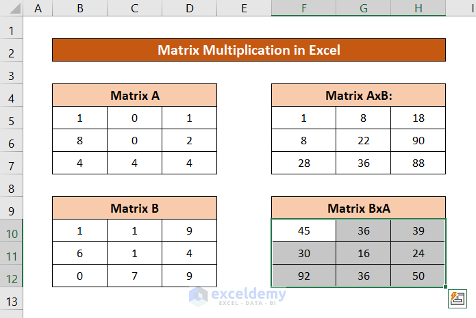
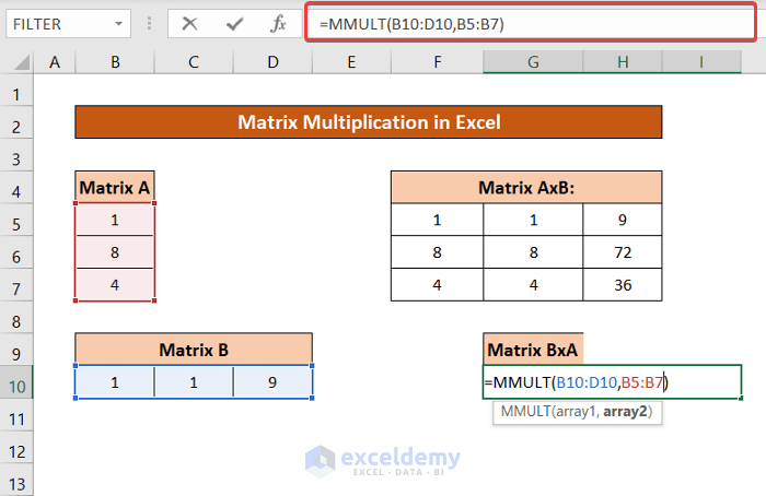
You can do the same for the BxA matrix by entering matrix B as the first argument and matrix A as the second argument of the MMULT function.

Method 2 – Multiplying One Column with One Row Array

The following dataset with matrices contains only one column and one row.

Steps:

• Select the range of cells for the multiplied matrix.

• Enter the following formula:

• Press Ctrl+Shift+Enter for the result.

Read More: How to Multiply Multiple Cells in Excel

Method 3 – Conducting One Row and One Column Array Multiplication in Excel

Steps:

• Select one cell.

• Enter the following formula:

• Press Ctrl+Shift+Enter for the result.

Read More: How to Multiply Rows in Excel

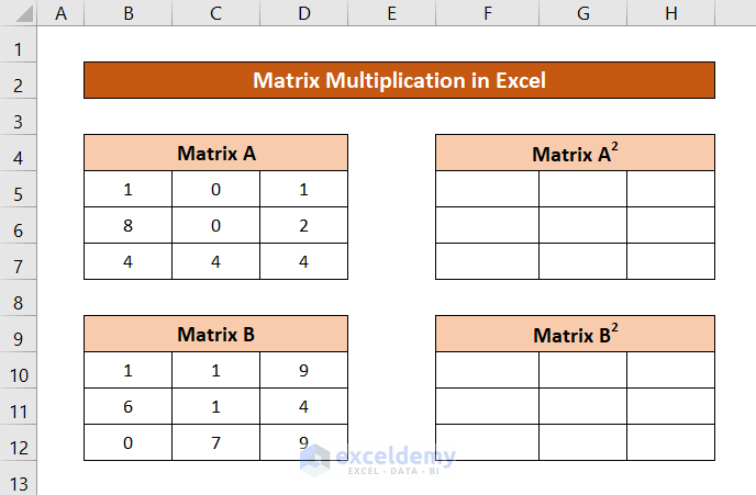
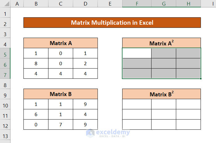
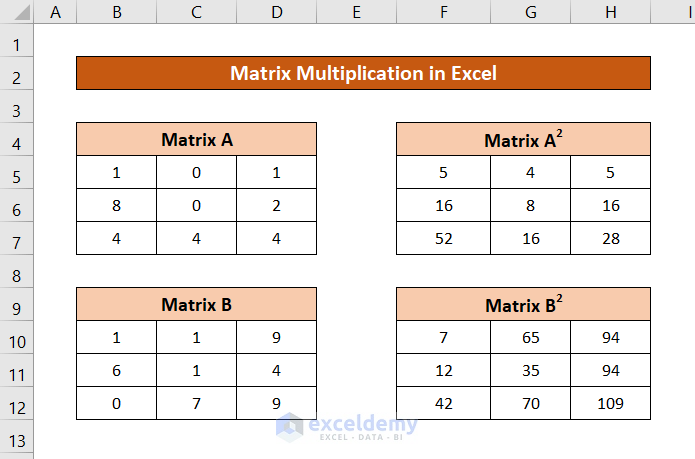
Method 4 – Calculating Square of a Matrix from Matrix Multiplication

Steps:

• Select the range of cells.

• Enter the following formula:

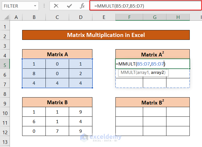
• Press Ctrl+Shift+Enter for the result.

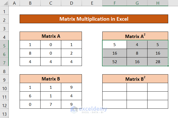
You can replace the range of matrix A with the range of matrix B (B10:D12) to get the square of matrix B.

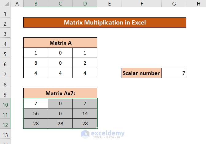
Method 5 – Doing Multiplication of a Matrix and a Scalar in Excel

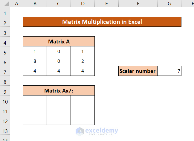
Steps:

• Select the range of cells.

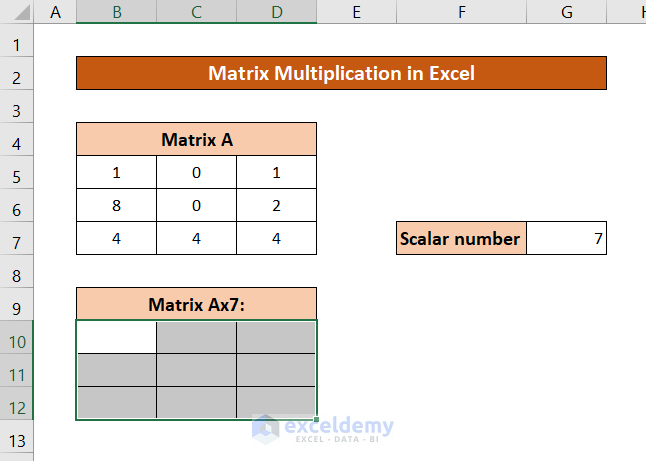
• Enter the following formula:

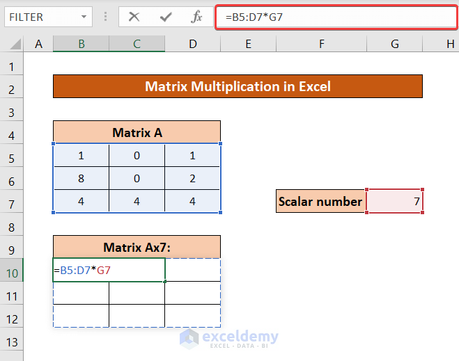
• Press Ctrl+Shift+Enter for the result.

Errors While Doing Matrix Multiplication in Excel

Look out for errors when applying matrix multiplication in Excel.

A common one is the #VALUE! error. This happens when the number of columns in the first array doesn’t match the number of rows in in the second array.

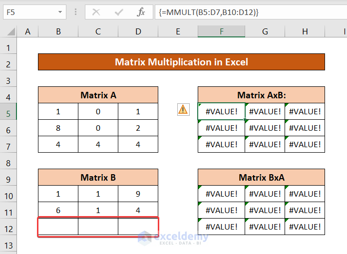
You will get the same #VALUE! error if there is at even one non-numeric value in a cell within the array.

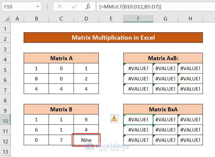
If you select more cells than what the multiplied matrix should be, you will get the #N/A error in the extra cells.

Download Practice Workbook

Related Articles

• How to Divide and Multiply in One Excel Formula
  
• How to Multiply from Different Sheets in Excel
• How to Create a Multiplication Formula in Excel 
• If Cell Contains Value Then Multiply Using Excel Formula 
• Multiply by Percentage in Excel 
• Multiply Two Columns and then Sum in Excel
• How to Multiply Two Columns in Excel
• How to Make Multiplication Table in Excel

<< Go Back to Multiply in Excel | Calculate in Excel | Learn Excel