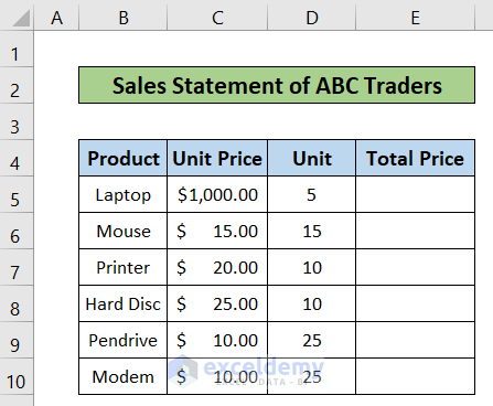
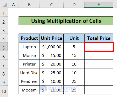
We will consider a dataset that has four columns, B, C, D, and E called Product, Unit Price, Unit, and Total Price.
Method 1 – Multiply Numbers to Create a Multiplication Formula in Excel
Steps:
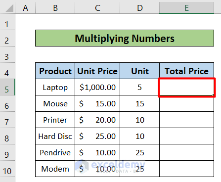
- Select the E5 cell of the dataset.
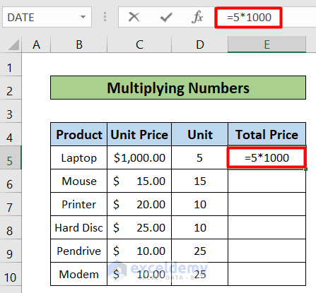
- Insert the following formula in the selected cell.
=5*1000Here, 5 is the unit value and 1000 is the unit price value.
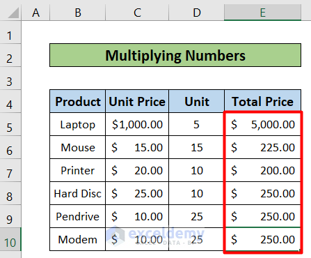
- For every cell, multiply the unit value by the unit price value.
Read More: How to Multiply Two Columns in Excel
Method 2 – Use Multiplication of Cells to Create a Multiplication Formula in Excel
Steps:
- Select the E5 cell.
- Enter the following formula in the selected cell.
=C5*D5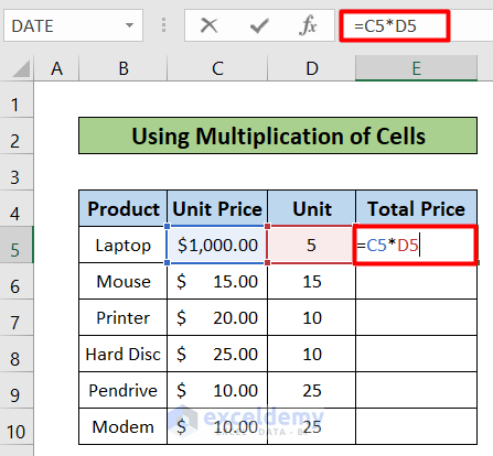
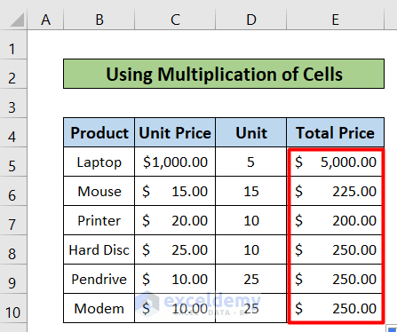
- Drag the Fill Handle of the formula from E5 to E10.

- You will get the total price of the products.
Read More: How to Multiply Multiple Cells in Excel
Method 3 – Multiply One Column by Another to Create a Multiplication Formula in Excel
Steps:
- Select the E5 cell of the dataset.

- Copy the following formula in the selected cell then.
=C5*D5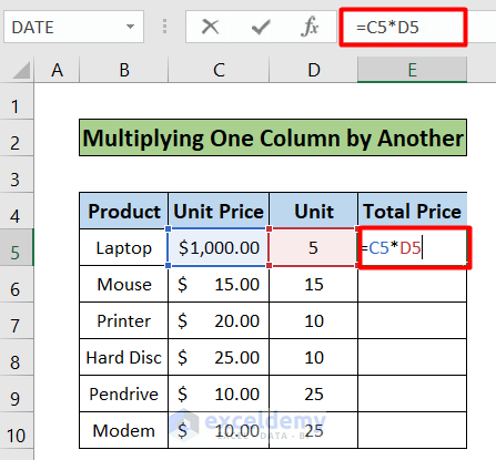
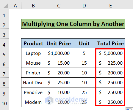
- Drag down the formula from E5 to E10.
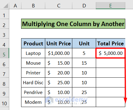
- You will find the result just like the picture below.
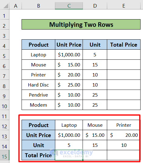
Method 4 – Creating a Multiplication Formula in Excel by Multiplying Two Rows
We have transposed the dataset for operation as we need to multiply two rows.
Steps:
- Select the C15 cell.
- Insert the following formula.
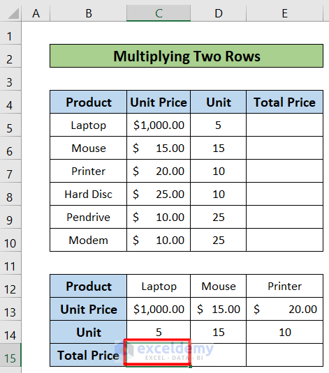
=C13*C14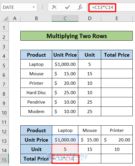
- Press Enter.
- Drag the formula from C15 to E15.
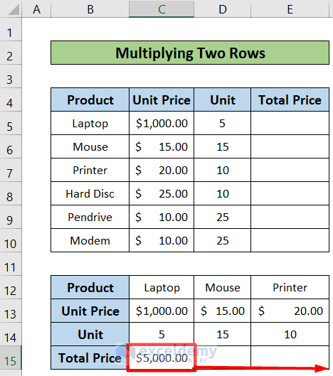
- You will find the following result.
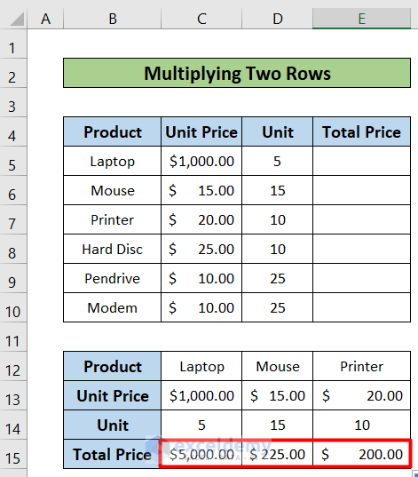
Read More: How to Multiply Rows in Excel
Method 5 – Use of the PRODUCT Formula to Create a Multiplication Formula in Excel
Steps:
- Select the E5 cell.
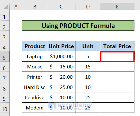
- Copy the following formula in the selected cell.
=PRODUCT(C5,D5)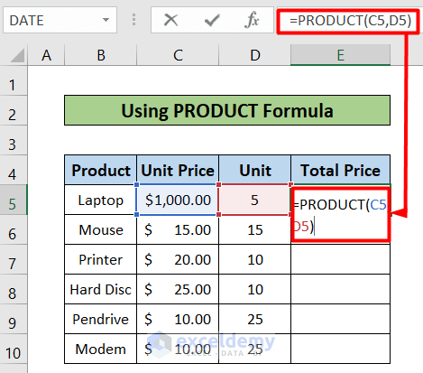
- Press Enter.
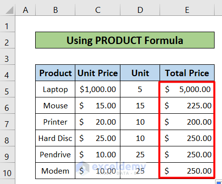
- Drag down the formula from E5 to E10 cells.
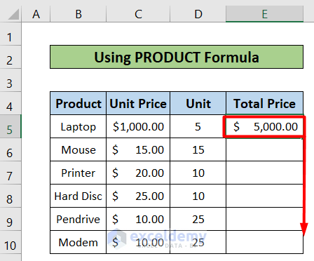
- You will find the result just like the picture given below.
How to Multiply a Cell by a Percentage
We have changed the dataset slightly. We will calculate the discounted amounts.
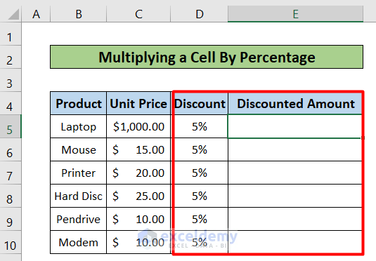
Steps:
- Select the E5 cell and copy the following formula.
=C5*D5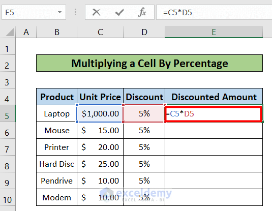
- Press the Enter button and drag down the formula from E5 to E10 cells.
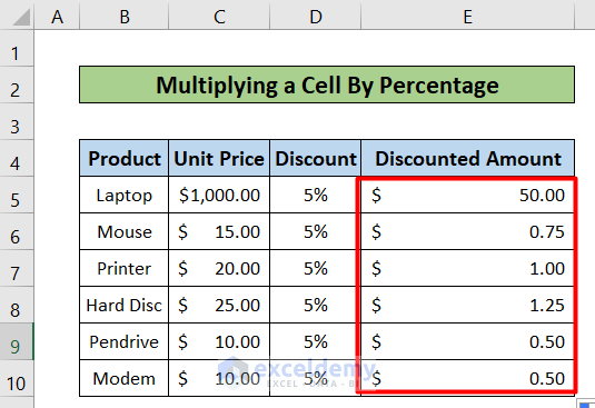
Read More: How to Multiply by Percentage in Excel
Multiplying a Column by Number
Steps:
- Select the E5 cell and write down the following formula.
=5*C5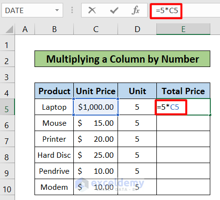
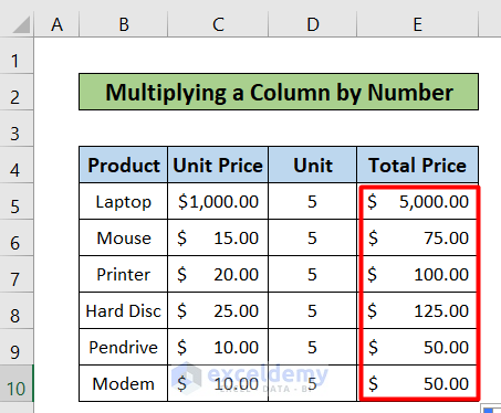
- After dragging down the formula, you will get the following result.
How to Multiply and Sum in Excel
Steps:
- Enter the following formula in the E5 cell first.
=C5*D5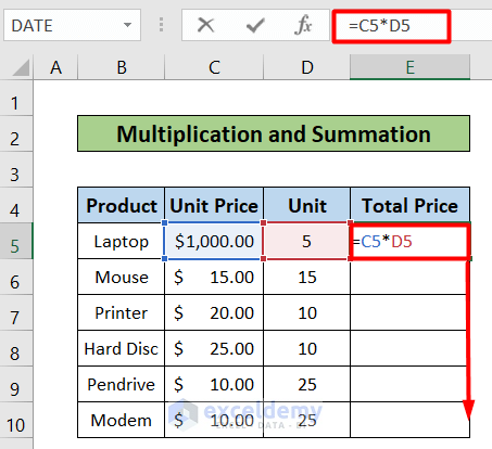
- After dragging down the formula you will get the following result.
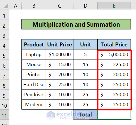
- In the E11 cell, copy the following formula.
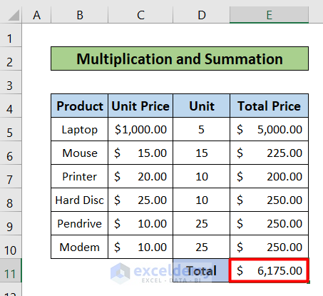
=SUM(E5:E10)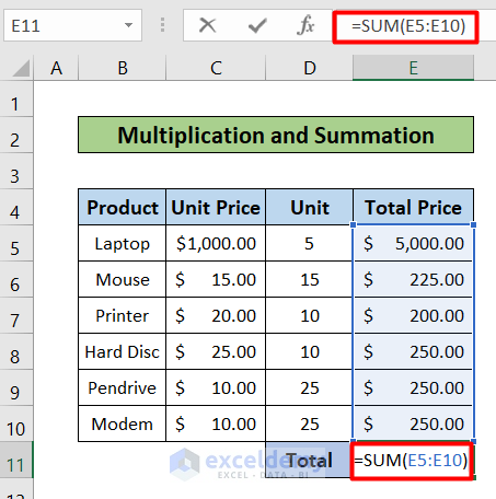
- You will find the total price just like the next picture.
Read More: How to Multiply Two Columns and Then Sum in Excel
Multiplication in Array Formulas
We will use the same dataset here.
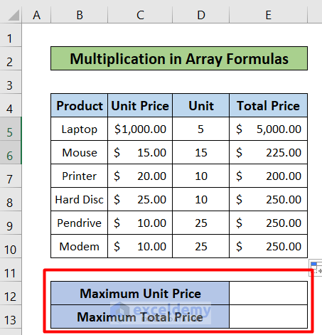
Steps:
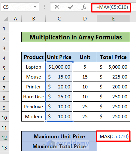
- Select the E12 cell and copy the following formula.
=MAX(C5:C10)- Press Enter.
- Use the following formula in the E13 cell.
=MAX(D5:D10*C5:C10)- Press Ctrl + Shift + Enter.
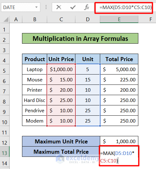
- You will find the result just like the following picture.
Download the Practice Workbook
Related Articles
- How to Divide and Multiply in One Excel Formula
- How to Do Matrix Multiplication in Excel
- How to Multiply from Different Sheets in Excel
- How to Make Multiplication Table in Excel
- If Cell Contains Value Then Multiply Using Excel Formula
<< Go Back to Multiply in Excel | Calculate in Excel | Learn Excel
Get FREE Advanced Excel Exercises with Solutions!

Great tips! I had no idea there were so many ways to create multiplication formulas in Excel. The step-by-step instructions made it really easy to follow. I’m definitely going to try using the array formula method. Thanks for sharing!
Hello,
You are most welcome. Thanks for your appreciation. Glad to hear that our step by step guide helped you to follow the instructions easily. Learn Excel with ExcelDemy!
Regards
ExcelDemy