Method 1 – Using the Keyboard Shortcut
Steps:
- Select the cell or cell range you want to shift down.
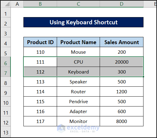
- Press the shortcut Ctrl+Shift+”+”.
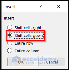
- The Insert box will pop up.
- Select Shift cells down in this box and click on OK.
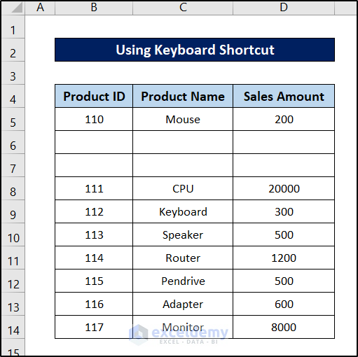
- The dataset will now look like this.
Read More: How to Shift Cells Right in Excel
Method 2 – Using the Context Menu
Steps:
- Select a cell or a range of cells.
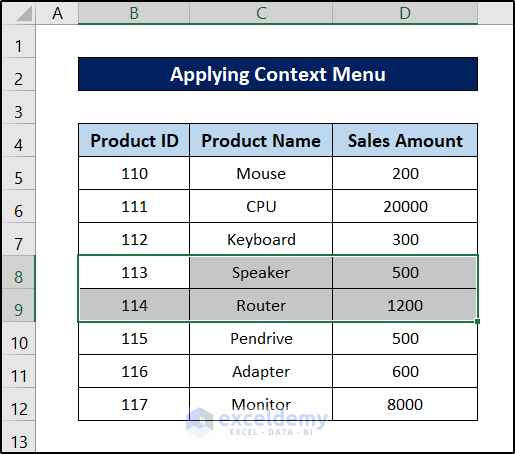
- Right-click on the selection.
- Choose the Insert option from the context menu.
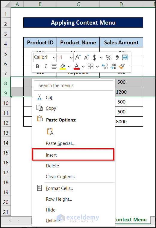
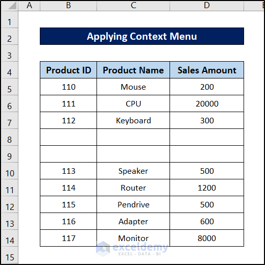
This will shift the cells down in the Excel spreadsheet.
Method 3 – Using the Insert Command from Cells Dropdown
Steps:
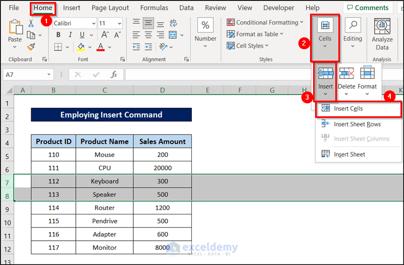
- Select a cell or cell range.
- Go to the Home tab.
- Select the Insert command from Cells.
- Select Insert Cells from the drop-down menu.
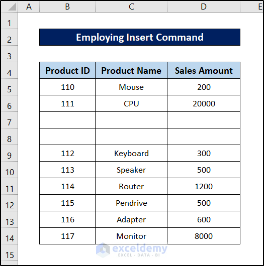
As a result, the cells will now shift down on the Excel spreadsheet.
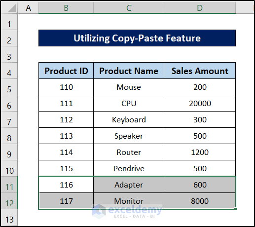
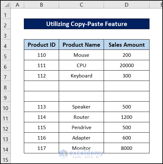
Method 4 – Using the Copy-Paste Feature
Steps:
- Select the cells you want to insert. Here, we are selecting the last two rows of the dataset.
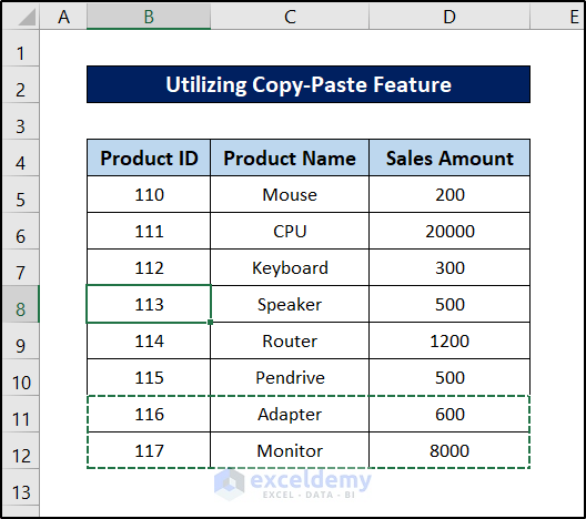
- Copy those cells by pressing Ctrl+C.
- Select any cell in the row above where you want to insert the copied cells (e.g., cell B8).
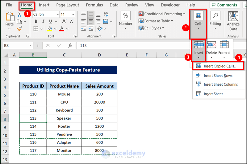
- Select Insert from the Cells group of the Home tab on your ribbon.
- Select Insert Copied Cells from the drop-down menu.
- Select Shift cells down from the Insert box and click on OK.
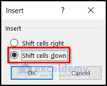
The cells are now copied into cell B8, and the rest of the cells have been shifted down.
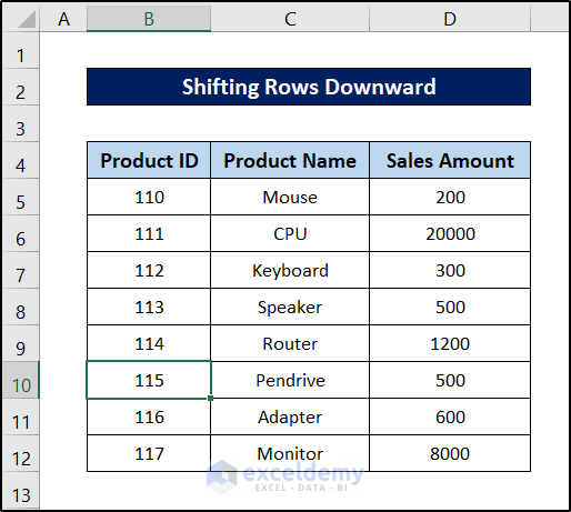
Method 5 – Shifting Rows Downward
Steps:
- Select any cell in the row above where you want another row (i.e., cell B10)
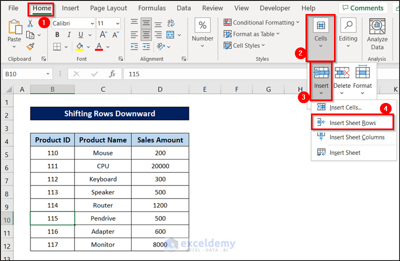
- Go to the Home tab on your ribbon.
- Select Insert from Cells.
- Select Insert Sheet Rows from the drop-down menu.
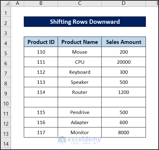
The new row has been inserted above the cell, and the rest of the cells have been shifted down.
Read More: How to Shift Cells Up in Excel
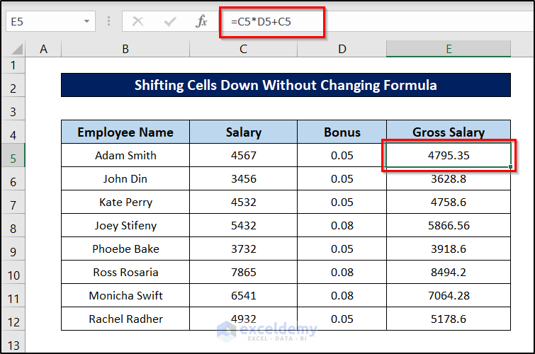
How to Shift Cells Down in Excel Without Changing the Formula
The following dataset contains formulas in column E.
Steps:
- Select the column you want to shift (i.e., range E5:E12).
- Move your cursor to the edge of the selection (not in the corners), and you will notice the cursor style changing.
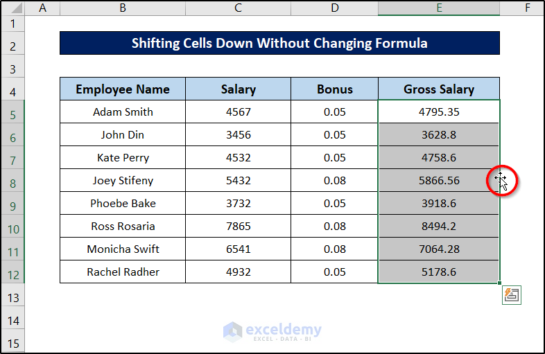
- Click on it and drag the cells down to where you want the range.
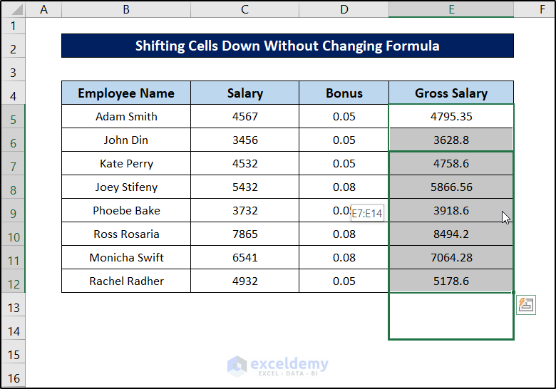
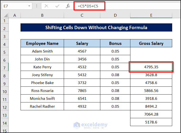
- Release the click.
This will shift these cells down in Excel without changing the formula.
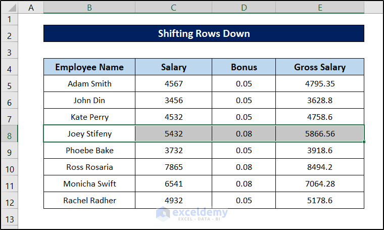
How to Shift Rows Down in Excel
Steps:
- Select the row you want to shift down.
- Hover your mouse over the border of the selection to notice the cursor style change.
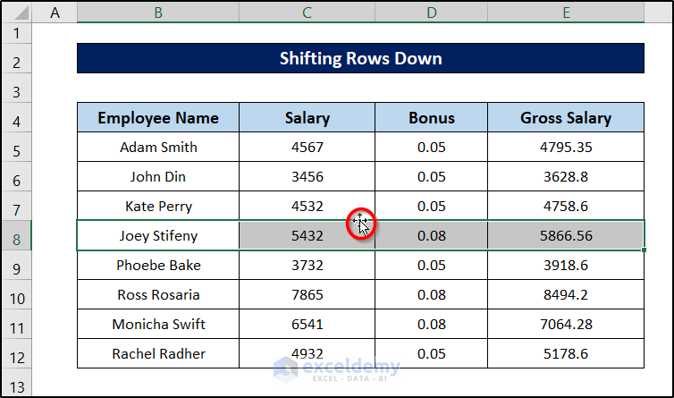
- Press Shift on your keyboard and click and drag the selection down to the position where you want the selection to be.
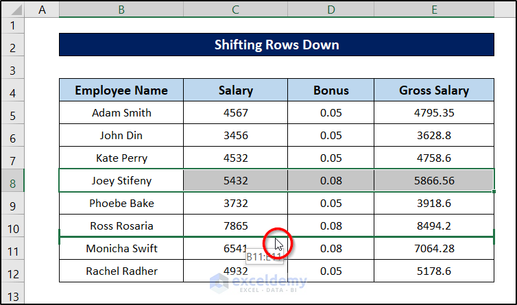
- Release the mouse.
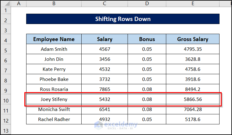
This will shift any number of selected rows down in Excel without creating new rows or changing the order of the other values in the dataset.
Download the Practice Workbook
You can download the workbook to practice.
Related Articles
- Fix: Excel Cannot Shift Nonblank Cells
- How to Perform Double Click Cell Jump in Excel
- How to Move Down One Cell Using Excel VBA
- Move One Cell to Right Using VBA in Excel
<< Go Back to Excel Cells | Learn Excel
Get FREE Advanced Excel Exercises with Solutions!

Alt+enter worked for me, but then a few hours later it doesn’t. When I press alt+enter it either opens a new book or closes the current one. Then I restarted my laptop and now it doesn’t do anything