In this article, we will let you know what mixed cell reference is in Excel and describe it with 4 examples.
What is Mixed Cell Reference in Excel?
Mixed cell reference in Excel is used when we want to lock
- either row while changing the columns
- or the column while changing the rows – when the formula is copied.
This can be done by simply putting the dollar ($) sign before the cell references.
Let’s understand the use of mixed cell reference with a simple multiplication table.
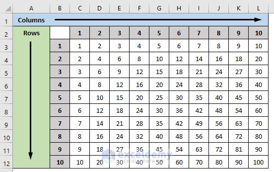
In the following example, we wrote the same numbers in columns and rows which we will be multiplying by mixed cell reference.

- To multiply each row with all the column values, we should lock the row by putting the dollar sign ($) in front of the row indexes and to multiply each column with all the row values, the dollar sign ($) should be in front of the column number to lock the column.
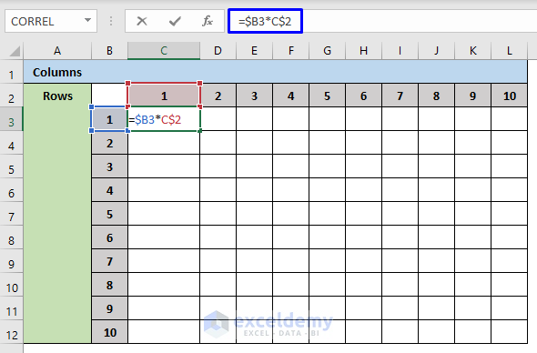
According to this, to calculate the multiplication table, the formula for the first cell will be,
=$B3*C$2- Press Enter and you will get the accurate result.
- To copy this formula in all the cells just drag the Fill Handle over the table and you will get the multiplication result using mixed cell references.
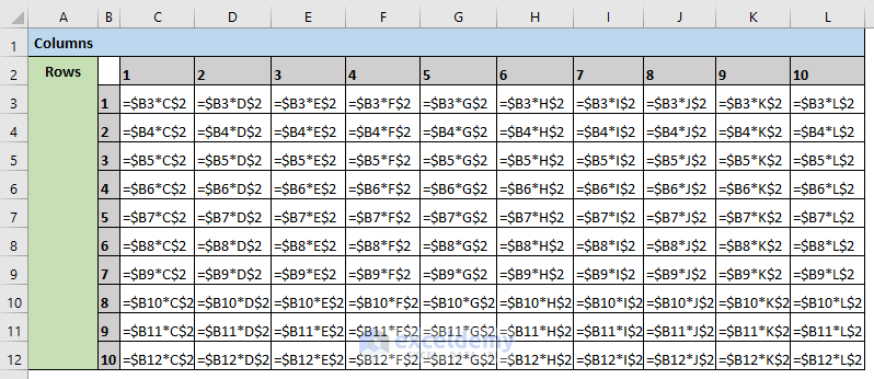
For your better understanding, we have provided formulas for the whole table for each cell.
Mixed Cell Reference in Excel: 4 Examples
This section describes 4 different examples of how to use the mixed cell reference in Excel.
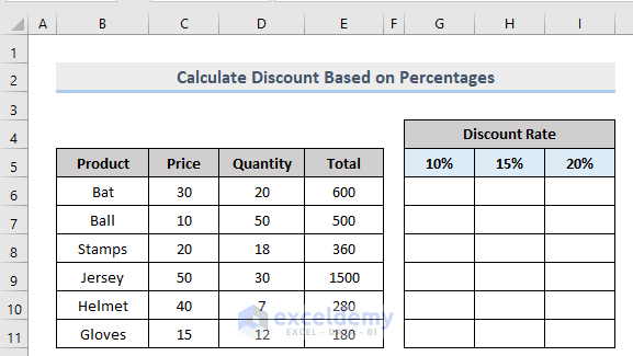
1. Calculate Discount Based on Percentages with Mixed Cell Reference in Excel
If you want to calculate discounts or commissions based on different percentage rates for specific products, then using the mixed cell reference is a very effective method in Excel.
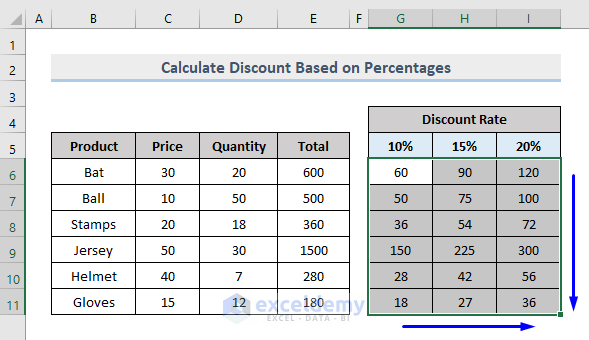
Look at the following example. Here we have to calculate the total discount amount for given products on 10%, 15% and 20% discount rates.
Let’s see how to do that with the mixed cell reference in Excel.
Steps:
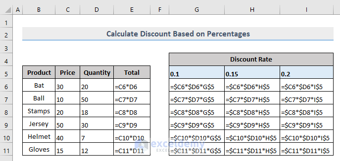
- In the Cell G6 (in our case, which is the cell to store the result), write the formula,
=$C6*$D6*G$5Here,
-> $C6 = the locked ($) Column C (column Price) with changing row number so that only the prices of the products will be inserted while calculating.
-> $D6 = the locked ($) Column D (column Quantity) with changing row number so that only the quantities of the products will be inserted while calculating.
-> G$5 = the locked ($) Row 5 (Discount Rate 10%) with changing column so that only the discount rates will be applicable while calculating the discount amount of different products.
- Press Enter. You will get the result according to your formula.

- Now drag the Fill Handle to apply the formula to the rest of the cells.
You can check the formulas for each cell from the picture below to understand the calculation with the mixed cell reference.
2. Compute Annual Income Tax Based on Tax Rates with Mixed Cell Reference
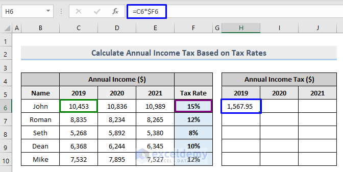
Here we will learn how to calculate annual income tax based on different tax rates on different years through mixed cell reference in Excel.

Let’s learn how to do that with the mixed cell reference in Excel.
Steps:
- In the Cell H6 (in our case, which is the cell to store the result), write the formula,
=C6*$F6Here,
-> C6 = value to calculate.
-> $F6 = the locked ($) Column F (column Tax Rate) with changing row number so that only the tax rates will be inserted while calculating.
- Press Enter. You will get the result according to your formula.
- Now drag the Fill Handle to apply the formula to the rest of the cells.
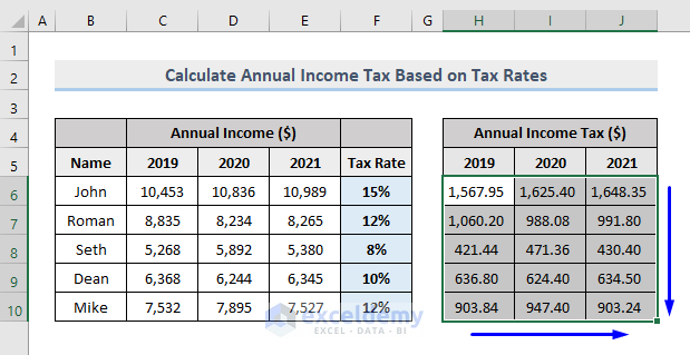
You can check the formulas for each cell from the picture below to understand the calculation with the mixed cell reference.

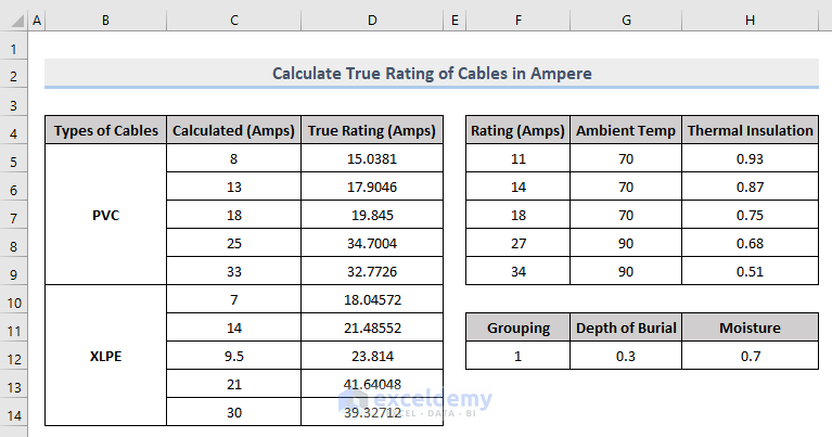
3. Determine the True Rating of Cables with Mixed Cell Reference in Excel
With Excel’s mixed cell reference you can also execute complicated calculations such as measuring the True Rating of cables in an Electrical Power System.
Suppose we have data as given below,
- Types of Cables
- Calculated Current in Ampere
- The details of the types of cables as
- Rating in Ampere
- Ambient temperature
- Thermal insulation
- Number of cable circuits running together
- Depth of the burial of the cable
- The moisture of the soil

With the given data, we will find out the true rating of cables using Excel’s mixed cell reference.
Steps:
- In the Cell D5 (in our case, which is the cell to store the result), write the formula,
=$F5*($G5/10)*$H5*F$12*G$12*H$12- Press Enter. You will get the result according to your formula.

- Now drag the Fill Handle through Cell D9 to apply the formula.
- You need to write the formula independently for the new type of cable in Cell D10. Here the formula is,
=$F5*($G5/10)*$H5*F$12*G$12*H$12*1.2- Press Enter. You will get the result according to your formula.
- Now drag the Fill Handle through Cell D14 to apply the formula.
We need to understand that to calculate the True Rating in Ampere from the given coefficient of Rating, Ambient Temp and Thermal Insulation, we must use the mixed cell reference because if we use Relative or Absolute Cell Reference it could lead to miscalculations due to non-uniform data distribution. To avoid this, we need to lock specific rows and columns according to our needs, hence using mixed cell reference to determine the Derating of Cables is a much more powerful method to utilize.
To understand the calculation for each cell with the mixed cell reference, you can check the formulas from the picture below.

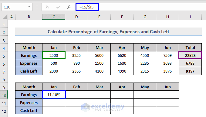
4. Measure the Percentage of Earnings, Expenses and Cash Left with Mixed Cell Reference
In this section, we will learn how to measure the percentage of Earnings, Expenses and Cash Left after Expenses against the Total of a company with the mixed cell references in Excel.
Let’s see how to do that with the mixed cell reference in Excel.
Steps:
- In the Cell C10 (in our case, which is the cell to store the result), write the formula,
=C5/$I5Here,
-> C5 = value to calculate.
-> $I5 = the locked ($) Column I (column Total) with changing row number so that only the total amount will be calculated against Earnings, Expenses and Cash Left.
- Press Enter. You will get the result according to your formula.
- Now drag the Fill Handle to apply the formula to the rest of the cells.
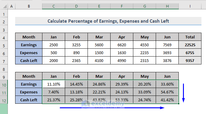
You can check the formulas for each cell from the picture below to understand the calculation with the mixed cell reference.

Download Workbook
You can download the free practice Excel workbook from here.
Conclusion
This article showed you 4 useful examples of mixed cell reference in Excel. I hope this article has been very beneficial to you. Feel free to ask if you have any questions regarding the topic.
Mixed Cell Reference in Excel: Knowledge Hub
<< Go Back to Cell Reference in Excel | Excel Formulas | Learn Excel
Get FREE Advanced Excel Exercises with Solutions!
