How to Insert a Dot between Numbers in Excel – 3 Methods

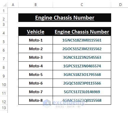
In the sample dataset, you have the Vehicle Engine Chassis Number, and want to insert dots.

Method 1 – Using the REPLACE Function to Insert a Dot between Numbers

Step 1:

• Insert the following formula in any cell (here, D5).

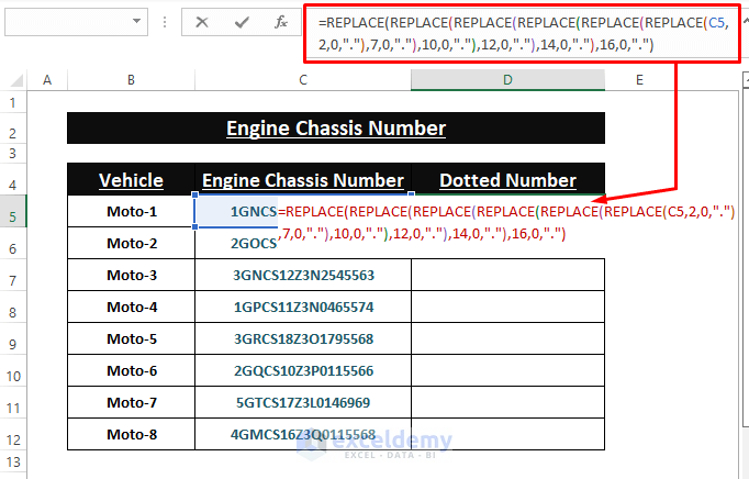
The formula takes the REPLACE function’s arguments ( old_text, start_num, num_chars, new_text). The multiple brackets insert dots in specific location.

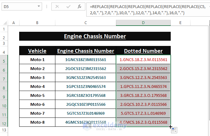
Step 2:

• Press ENTER and drag the Fill Handle.

Method 2 – Inserting Dots between Numbers Using Multiple Formulas

Step 1:

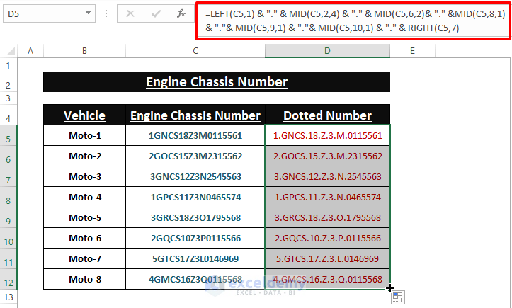
• Enter the following formula in D5.

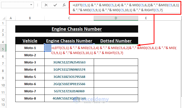The formula inserts the 1^st dot using the LEFT function and the middle dots using the MID function. The  RIGHT function inserts the last dot.

Step 2:

• Press ENTER and drag the Fill Handle.

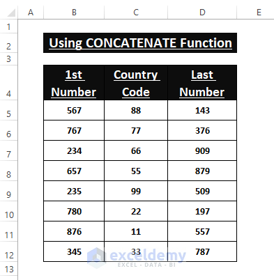
Method 3 – Using the CONCATENATE Function to Insert Dots within Numbers in Excel

To create Unique Ids with dots.

Step 1:

• Enter the formula in E5.

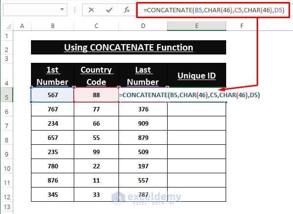
The CONCATENATE function takes multiple texts as arguments (iB5, CHAR (46),….) to concatenate them as a Unique Id. The CHAR function represents the ASCII code for the Dot character.

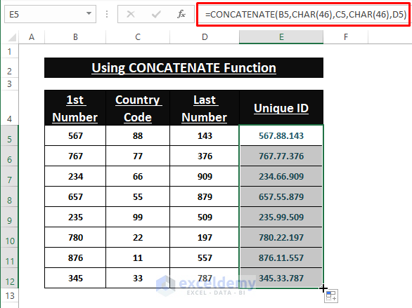
Step 2:

• Press ENTER key to apply the formula and drag the Fill Handle.

Using Cell Formatting to Insert a Trailing Dot

Step 1:

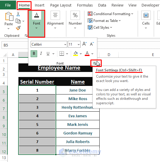
• Select the entire column.
• Go to the Home tab to and in Font, choose Font Settings or press CTRL+1, to open the Format Cells window.

Step 2:

• In the Format Cells window. Go to Number  > Select Custom (under Category) > In Type, enter #. Click OK.

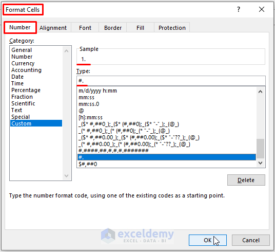
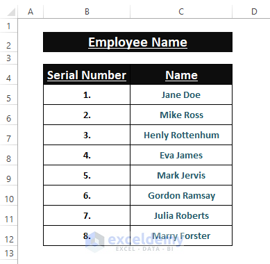
The column displays trailing dots.

Download Excel Workbook

Related Article

•  How to Add Dashes to SSN in Excel

<< Go Back to Bullets and Numbering in Excel | Worksheet Formatting | Learn Excel