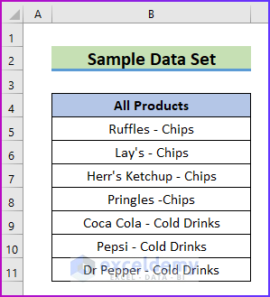
This is the sample dataset.
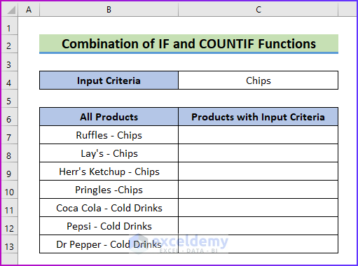
Method 1 – Combining the IF and the COUNTIF Functions
Steps:
- Prepare a dataset.
- To find cells containing a specific word mentioned in the Criteria header in C4:
- Enter the following formula in C7.
=IF(COUNTIF($B7,"*"&$C$4&"*"), B7, "Not Found")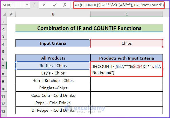
Formula Breakdown
=IF(COUNTIF($B7,”*”&$C$4&”*”), B7, “Not Found”)
- IF(COUNTIF($B7,”*”&$C$4&”*”), B7, “Not Found”): the asterisk sign (*) is a wildcard character. It searches for “Chips” substring within B7.
- The COUNTIF function returns one for every substring match.
- The value of the IF function is one (1)=TRUE, it returns the first argument: the desired output.
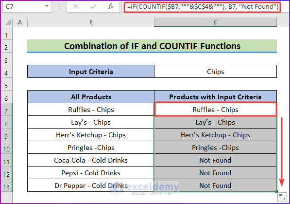
- Press Enter.
- Drag down the Fill Handle to see the result in the rest of the cells.
Method 2 – Merging the IF, ISNUMBER, and SEARCH Functions
Steps:
- Set the input criteria in C4.
- Enter the formula in C7.
=IF(ISNUMBER(SEARCH($C$4,$B7)),B7,"Not Found")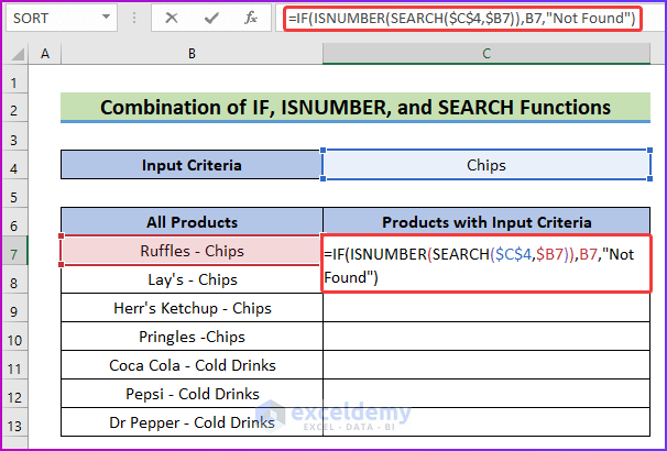
Formula Breakdown
=IF(ISNUMBER(SEARCH($C$4,$B7)),B7,”Not Found”)
- IF(ISNUMBER(SEARCH($C$4,$B7)),B7,”Not Found”): the SEARCH function searches the value of the input criteria in B7. For “Chips”, it returns 11, which is the starting position of the substring.
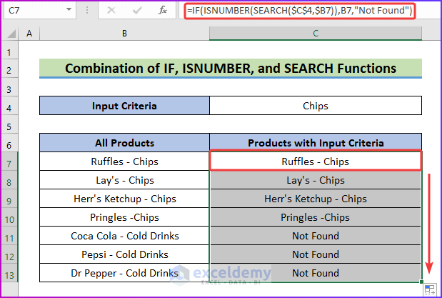
- The ISNUMBER function converts 11 into TRUE.
- As the IF function’s value is TRUE, it returns the first argument: the desired output.
- Press Enter to see the result.
- Drag down the Fill Handle to see the result in the rest of the cells.
Method 3 – Combine the IF, ISNUMBER and FIND Function
Steps:
- Set the input criteria in B7.
- Enter the formula in C7.
=IF(ISNUMBER(FIND($C$4,$B7)), B7, "Not Found")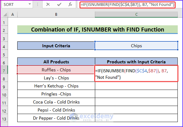
Formula Breakdown
=IF(ISNUMBER(FIND($C$4,$B7)), B7, “Not Found”)
- IF(ISNUMBER(FIND($C$4,$B7)), B7, “Not Found”): The FIND function searches the value of the input criteria in B7 and returns the location. For “Chips” it returns 11, which is the starting position of the substring.
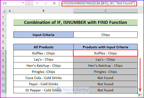
- The ISNUMBER function converts 11 into TRUE.
- As the IF function’s value is TRUE, it returns the first argument: the desired output.
- Press Enter to see the result.
- Drag down the Fill Handle to see the result in the rest of the cells.
Method 4 – Combine the VLOOKUP Function with the IF and IFERROR Functions
Steps:
- Enter the formula in C7.
=IFERROR(IF(VLOOKUP($C$4,$B7,1,TRUE)="Chips", B7, B7),"Not Found")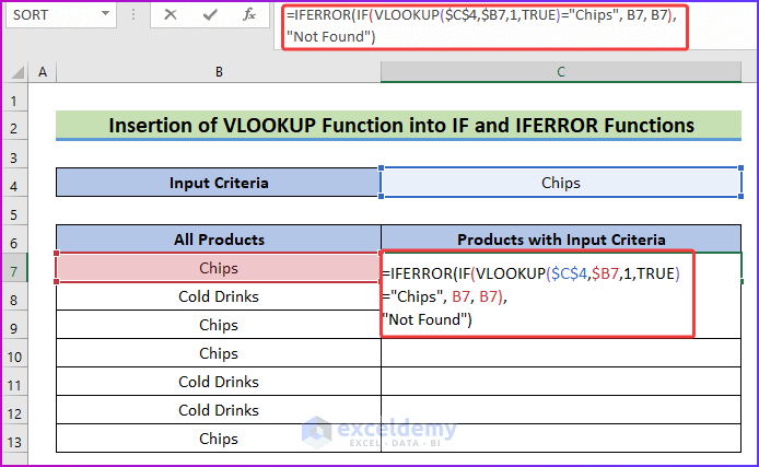
Formula Breakdown
=IFERROR(IF(VLOOKUP($C$4,$B7,1,TRUE)=”Chips”, B7, B7),”Not Found”)
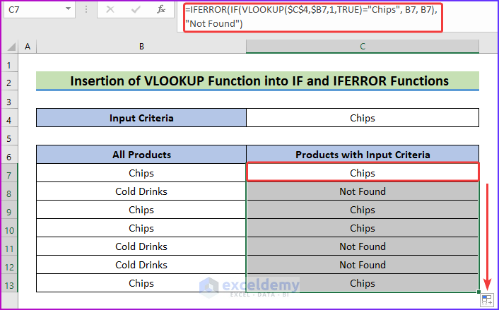
- IFERROR(IF(VLOOKUP($C$4,$B7,1,TRUE)=”Chips”, B7, B7),”Not Found”): , the VLOOKUP function looks up the criteria Chips in B7 and returns the cell’s value, which is Chips.
- the IF function returns the value of the cell: Chips.
- As the IFERROR function’s first argument is not an error, it returns the value: the desired output.
- Press Enter to see the result.
- Drag down the Fill Handle to see the result in the rest of the cells.
Download Practice Workbook
<< Go Back to Text | If Cell Contains | Formula List | Learn Excel
Get FREE Advanced Excel Exercises with Solutions!

Thank you so much on the Using the COUNTIF function! Can’t get easier to me.