Method 1 – Converting Commas to Decimal Points to Remove Commas from Numbers
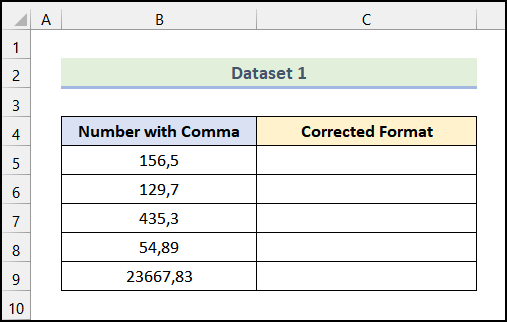
The following dataset contains Numbers with Commas. To convert the commas to decimal points:
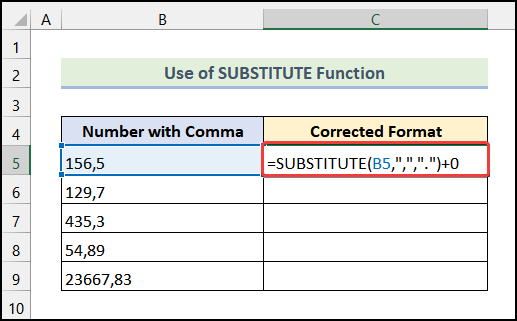
1.1 Using SUBSTITUTE Function
Steps:
- Enter the following formula in B5.
=SUBSTITUTE(B5,",",".")+0- Press ENTER.
Note: 0 was added after the SUBSTITUTE function to display the Number Format.
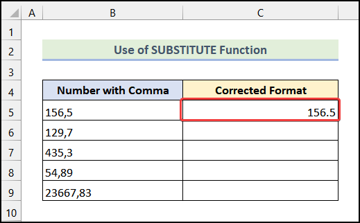
This is the output.
Note: As the number is no longer in Text Format, it is now right aligned.
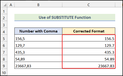
- Use the AutoFill feature to see the result in the rest of the cells.
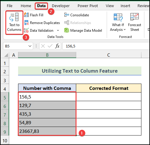
1.2 Utilizing the Text to Columns Feature
Steps:
- Select the data to apply the Text to Columns feature.
- Go to the Data tab.
- Click Text to Columns.
The Convert Text to Columns Wizard will open.
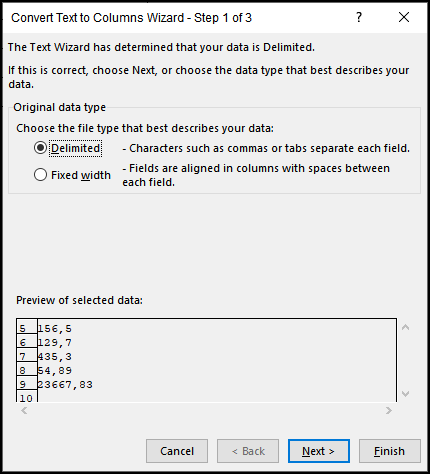
- Select Fixed width and click Next.
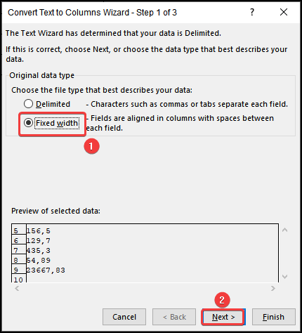
- Click Next again.
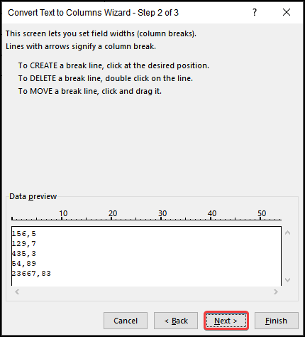
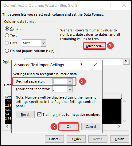
- Click Advanced.
- Enter a comma (,) in Decimal separator.
- Click OK.
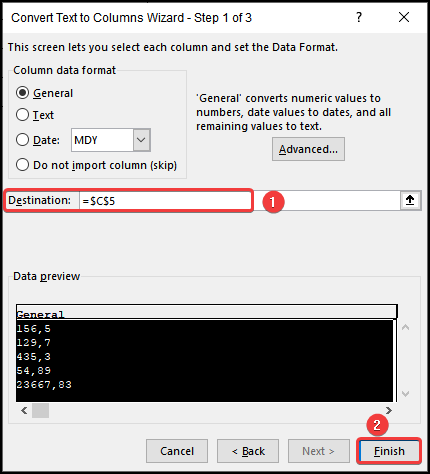
- In Destination, select C5.
- Click Finish.
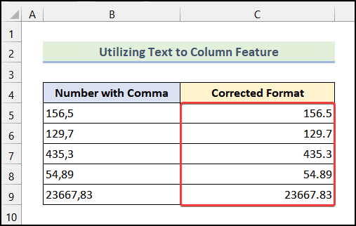
This is the output.
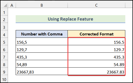
1.3 Using the Find & Replace Feature of Excel
Steps:
- Copy the cells of the Number with Comma column and paste them into the Corrected Format column.
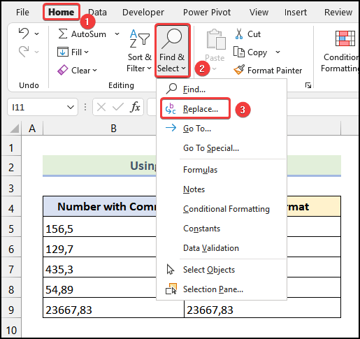
- Go to the Home tab.
- Choose Find & Select in Editing.
- Select Replace.
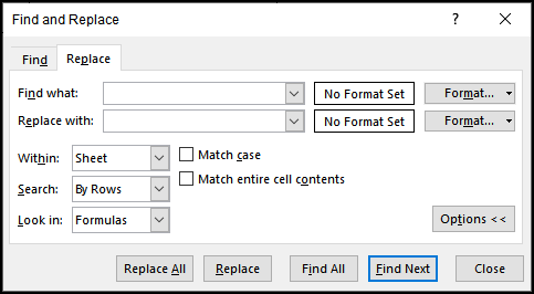
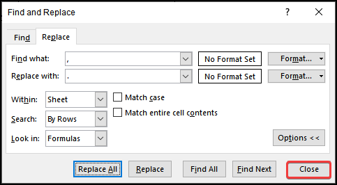
The Find and Replace dialog box will open.
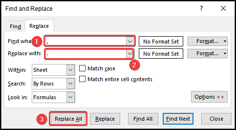
- In Find what, enter comma (,) and in Replace with, enter decimal point (.).
- Click Replace All.
- Excel will show a message: All done. We made 5 replacements. Click OK.
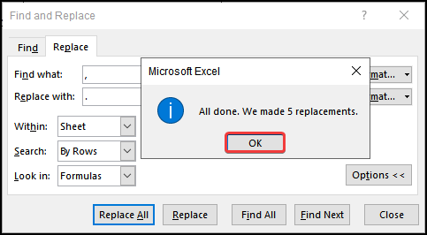
- Click Close.
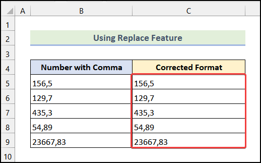
Commas are removed and replaced with a decimal point.
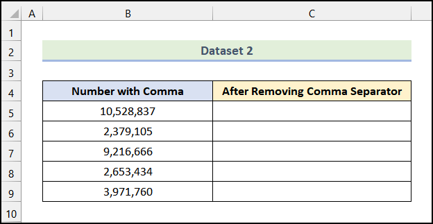
Method 2 – Removing Thousands Comma Separators from Numbers
In the following dataset there are numbers which have thousands comma separators.
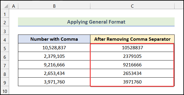
2.1 Applying the General Format
Steps:
- Copy the cells of the Number with Comma column and paste them into the After Removing Comma Separator column.
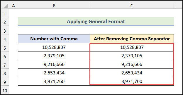
- Select the After Removing Comma Separator column.
- Go to the Home tab.
- Click Number and choose General.
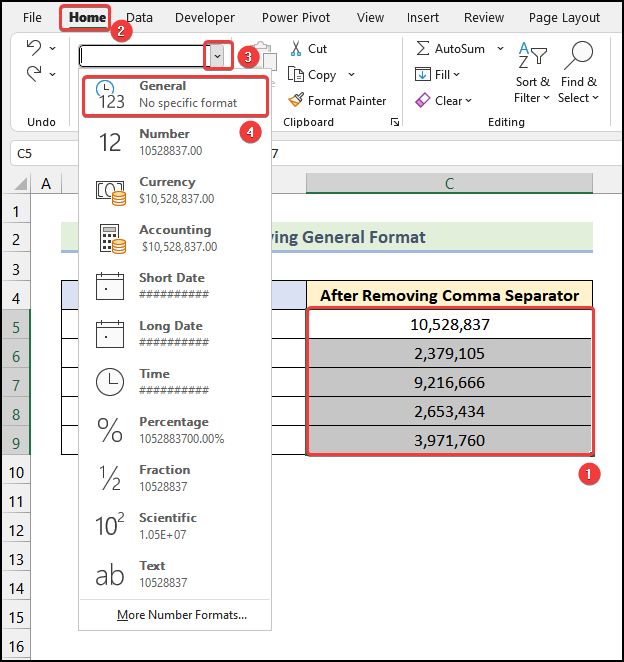
This is the output.
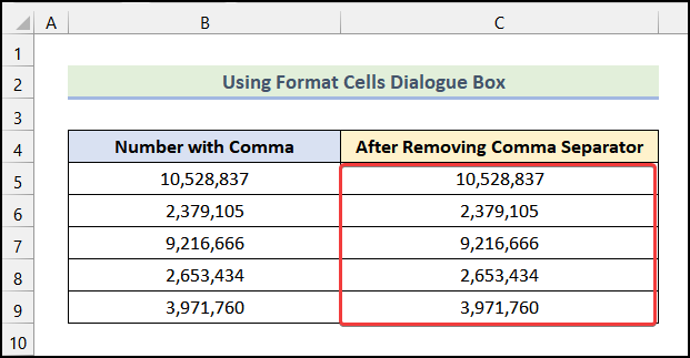
2.2 Using the Format Cells Dialog Box
Steps:
- Copy the cells of the Number with Comma column and paste them into the After Removing Comma Separator column.
- Select the After Removing Comma Separator column.
- Click as shown below.
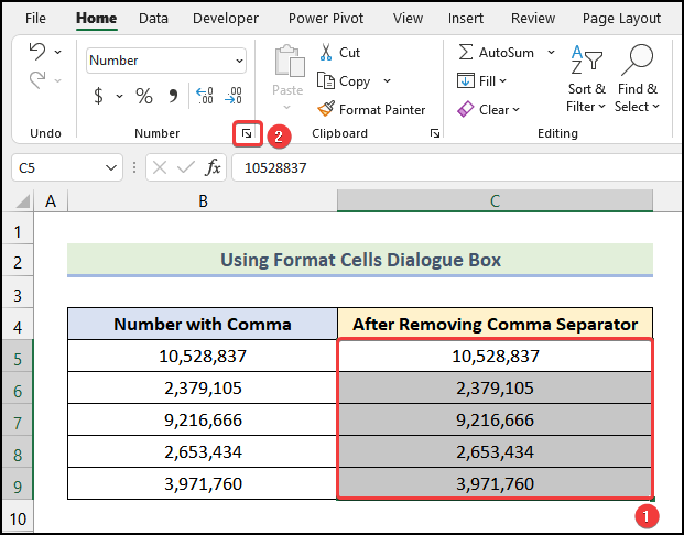
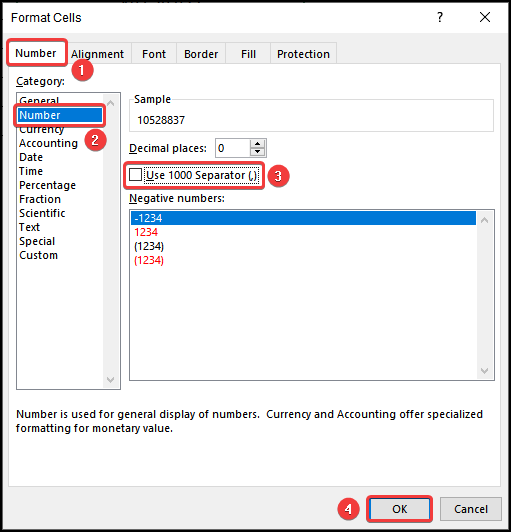
The Format Cells dialog box will be displayed.
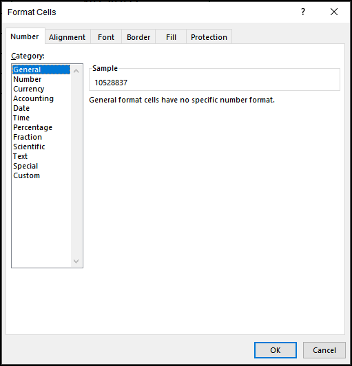
Note: You can press CTRL + 1 to open the Format Cells dialog box.
- Click Number.
- Uncheck Use 1000 separator (,).
- Click OK.
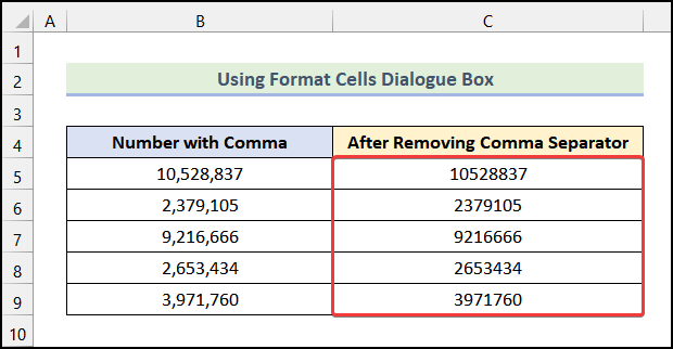
This is the output.
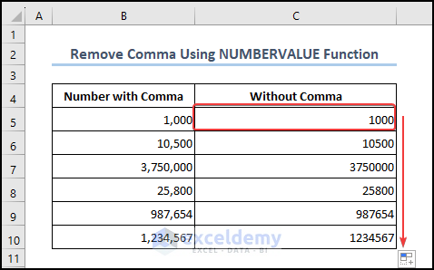
2.3 Using the NUMBERVALUE Function to Remove Commas
Steps:
- Use the following formula in C5 and press ENTER.
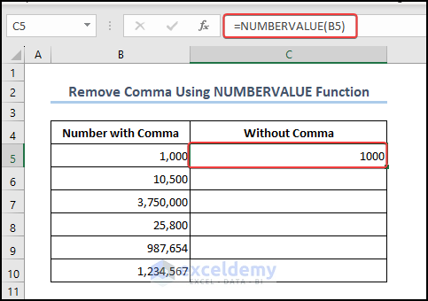
- Drag down the Fill Handle to see the result in the rest of the cells.
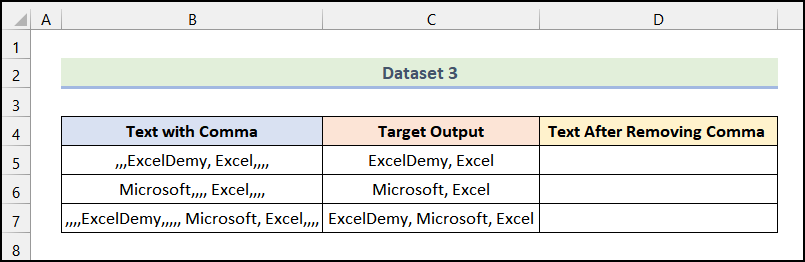
Method 3 – Deleting Commas in Texts
3.1 Using the SUBSTITUTE and the TRIM Functions
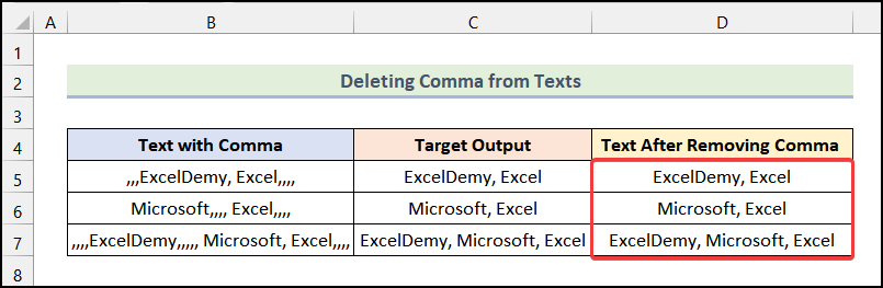
The following dataset contains Text with Commas and the Target Output.
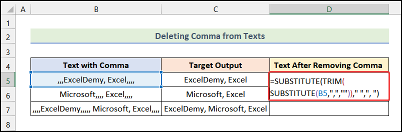
Steps:
- Enter the following formula, in D5.
=SUBSTITUTE(TRIM(SUBSTITUTE(B5,",",""))," ",", ")Formula Breakdown
- SUBSTITUTE(B5,”,”,””) → replaces all commas with blanks. It converts “,,,ExcelDemy, Excel,,,,” to “ ExcelDemy Excel “.
- TRIM(” ExcelDemy Excel “) → returns: “ExcelDemy Excel“
- =SUBSTITUTE(“ExcelDemy Excel”,” “,”, “) → replaces the Spaces with a comma and Space.
- Output → ExcelDemy, Excel.
- Press ENTER.
This is the output.
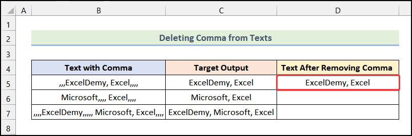
- Drag down the Fill Handle to see the result in the rest of the cells.
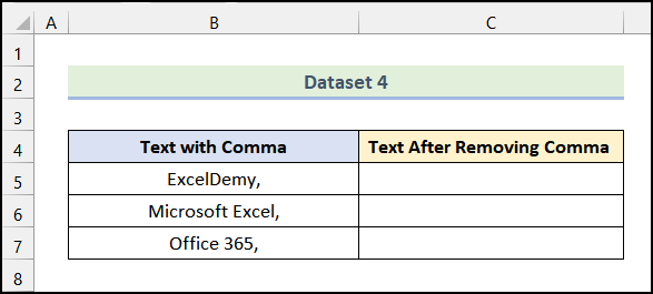
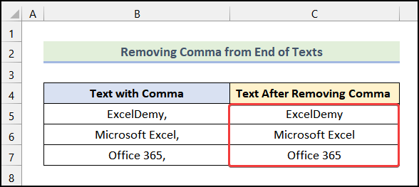
Method 4 – Removing Commas at the End of Texts in Excel
To remove the comma at the end of the texts:
Steps:
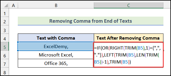
- Use the following formula in C5.
=IF(OR(RIGHT(TRIM(B5),1)={",","."}),LEFT(TRIM(B5),LEN(TRIM(B5))-1),TRIM(B5))Formula Breakdown
- logical_test of the IF Function: OR(RIGHT(TRIM(B5),1)={“,”,”.”}). The TRIM function (TRIM(B5)) removes all extra spaces. RIGHT(returned_text_by_TRIM,1), returns the rightmost character from the trimmed text. OR(right_most_character_of_trimmed_text={“,”,”.”}), returns TRUE if the rightmost character is a comma or a period. Returns FALSE if the rightmost character is not a comma or a period. For “Exceldemy, “, TRUE.
- value_if_true of the IF function: LEFT(TRIM(B5),LEN(TRIM(B5))-1)
- We can simplify this formula: LEFT(trimmed_text,length_of_the_trimmed_text-1). It returns the whole trimmed text except for the last character.
- value_if_false of the IF function: TRIM(B5)
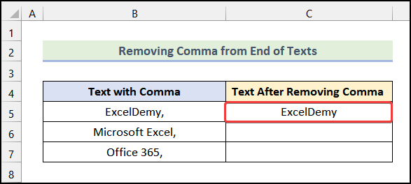
- Output → ExcelDemy.
- Press ENTER.
This is the output.
- Drag down the Fill Handle to see the result in the rest of the cells.
How to Remove Numbers after a Comma in Excel
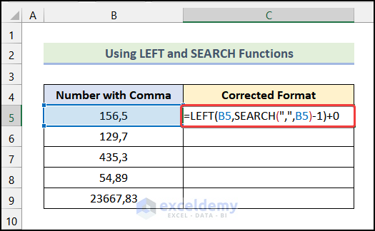
Using the LEFT and the SEARCH Functions
Steps:
- Enter the formula in C5.
=LEFT(B5,SEARCH(",",B5)-1)+0Formula Breakdown
- SEARCH(“,”,B5)-1) → returns the position of the comma (,) in the text in B5. The position is 4.
- The LEFT function, returns the first 3 characters.
- At the end of the formula, 0 turns the value to a number.
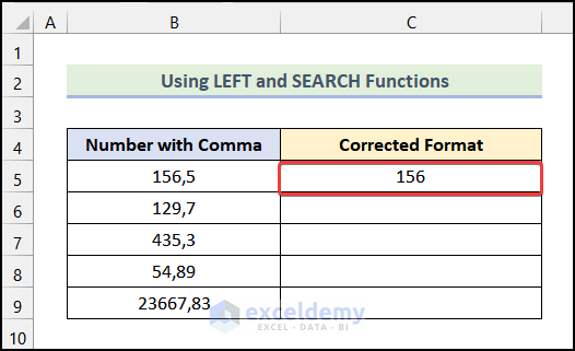
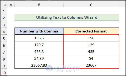
- Output → 156.
- Press ENTER.
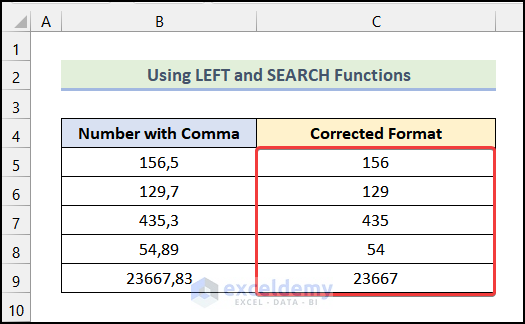
This is the output.
- Drag down the Fill Handle to see the result in the rest of the cells.
♦ Utilizing the Text to Columns Wizard
Steps:
- Follow the steps described above.

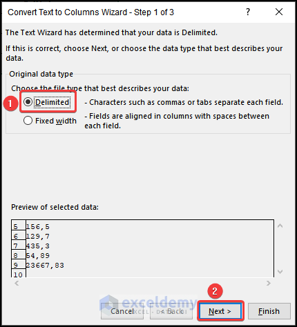
- In the Convert Text to Columns Wizard, choose Delimited and click Next.
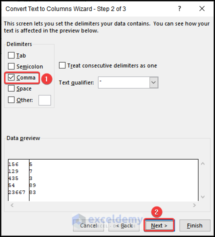
- Check Comma and click Next.
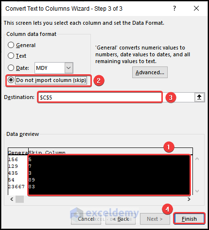
- Select the column as shown below.
- Choose Do not import column (skip).
- Select C5 as destination.
- Click Finish.
This is the output.
Things to Remember
- You may use Ctrl+H to open the Find and Replace dialog box.
Frequently Asked Questions
1. How do I remove 3 characters from left in Excel?
Use the REPLACE function.
2. How do I separate names in Excel with commas?
Use the Text to Column feature.
3. What is the disadvantage of using the Text to Columns Wizard to remove commas in Excel for numbers?
The resulting value is not a number.
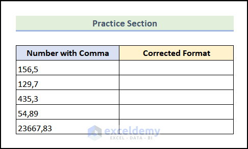
Practice Section
Practice here.
Download Practice Workbook
Get FREE Advanced Excel Exercises with Solutions!
