


In Excel, single-criteria lookups like basic VLOOKUP or XLOOKUP are common, but real-world data often requires matching on multiple conditions at once, like “find the price for this product AND this size AND this region.” Excel does not have a separate “multi-criteria lookup” function. Instead, you can combine logical conditions inside XLOOKUP or INDEX/MATCH.
In this tutorial, we will show how to perform multi-criteria lookups with XLOOKUP and INDEX/MATCH. While older Excel versions relied on complex formulas, modern Excel makes these lookups much easier, especially with XLOOKUP.
Method 1: XLOOKUP with Concatenated Keys
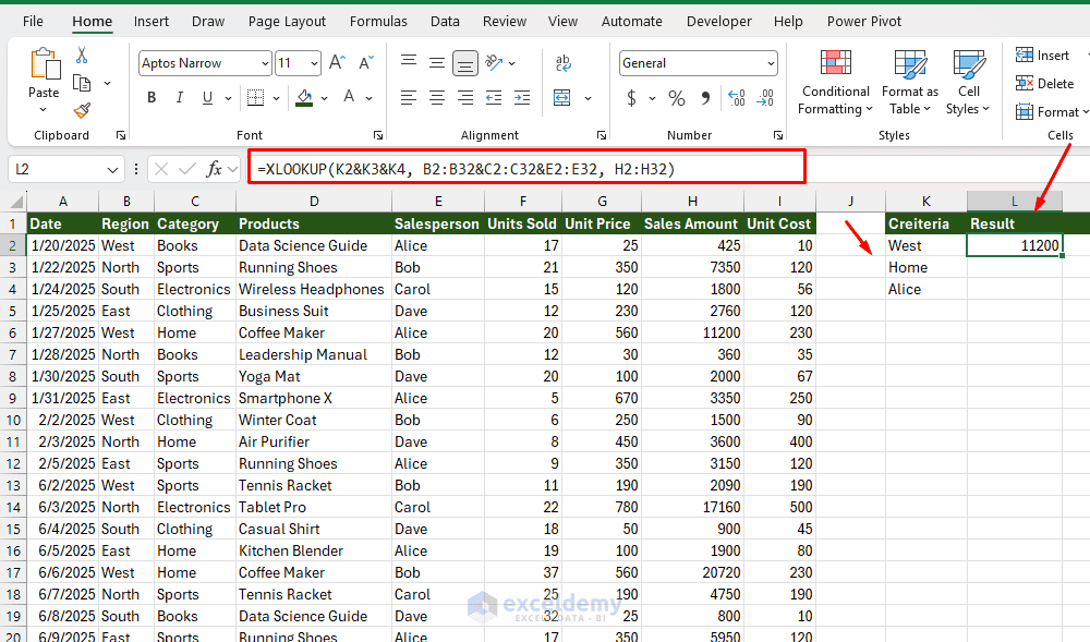
XLOOKUP natively only takes one lookup array, so you need to build a combined key by joining criteria with &.
=XLOOKUP(K2&K3&K4, B2:B32&C2:C32&E2:E32, H2:H32)
Here, K2, K3, and K4 contain the criteria; based on these criteria, XLOOKUP searches and returns the sales amount. B2:B32&C2:C32&E2:E32 creates an array like {“WestHomeAlice”, “Widget NorthSportBob”, …} in memory. XLOOKUP then matches this against your concatenated search key K2&K3&K4.
Use a Delimiter: Avoid joining criteria without a separator.
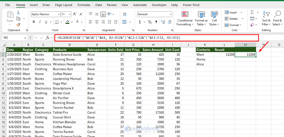
Concatenation can accidentally match different combinations that produce the same string (e.g. “AB”&”C” = “A”&”BC”). Add a delimiter to be safe:
=XLOOKUP(K2&"|"&K3&"|"&K4, B2:B32&"|"&C2:C32&"|"&E2:E32, H2:H32)
Handle errors gracefully:
=XLOOKUP(K2&"|"&K3&"|"&K4, B2:B32&"|"&C2:C32&"|"&E2:E32, H2:H32, "Not Found")
This formula works across multiple conditions, and if no match is found, it returns “Not Found” instead of a #N/A error.
Important: This is an array formula. In modern Excel (365/2021+), it spills automatically. In older versions, press Ctrl+Shift+Enter.
Method 2: XLOOKUP with Boolean Multiplication
A cleaner alternative avoids string concatenation entirely by multiplying TRUE/FALSE conditions.
=XLOOKUP(1, (B2:B32=K2)*(C2:C32=K3)*(E2:E32=K4), H2:H32)
Each condition, like (B2:B32=K2), returns an array of TRUE/FALSE values. Multiplying these arrays converts them to 1/0, and only the row where all three conditions are TRUE (1×1×1=1) produces a 1. XLOOKUP then searches for that 1.
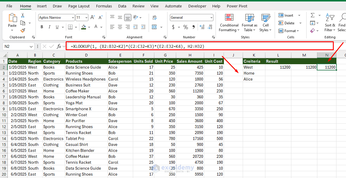
This method is generally safer than concatenation since there is no risk of string-boundary false matches, and it reads more like “match all these conditions” once you are used to the pattern.
Method 3: INDEX/MATCH with an Array Match
The classic pre-XLOOKUP approach is still fully valid and often preferred for compatibility with older files.
=INDEX(H2:H32, MATCH(1, (B2:B32=K2)*(C2:C32=K3)*(E2:E32=K4), 0))
This uses the same boolean logic as Method 2, but INDEX/MATCH separates “find the row number” (MATCH) from “return the value in that row” (INDEX). The 0 in MATCH forces an exact match.
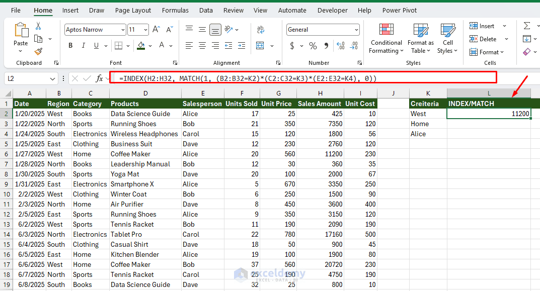
In older versions of Excel, this also requires Ctrl+Shift+Enter. If you see {…} braces around the formula in the formula bar, it has been entered correctly as an array formula.
Bonus: Returning Multiple Columns at Once
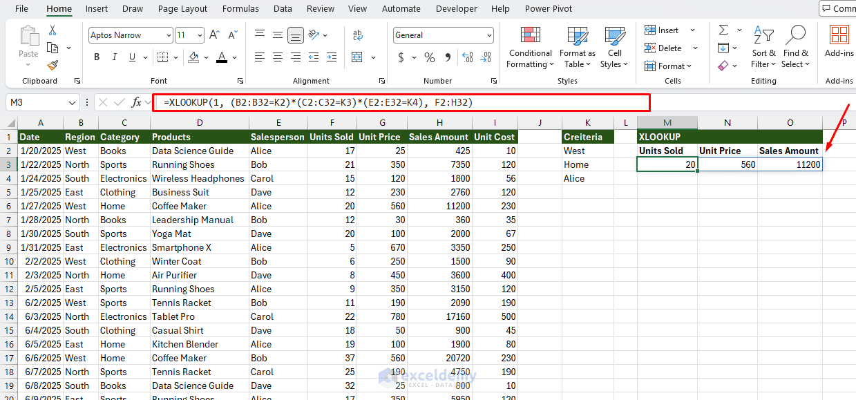
XLOOKUP lets you return more than one column in a single formula, which is useful if you want Size and Price together.
=XLOOKUP(1, (B2:B32=K2)*(C2:C32=K3)*(E2:E32=K4), F2:H32)
This automatically spills both Unit and Price into adjacent cells (Excel 365 only).
Which Method Should You Use?
| Situation | Recommended Method |
| Excel 365 / 2021+, want cleanest syntax | XLOOKUP + Boolean multiplication |
| Sharing a file with users on older versions of Excel | INDEX/MATCH with array match |
| Need to return multiple columns at once | XLOOKUP with a multi-column return range: =XLOOKUP(1,(B2:B32=K2)*(C2:C32=K3),E2:H32) |
| Criteria include numbers with possible blanks | Boolean method (avoids blank-concatenation issues) |
Common Errors and Fixes
| Error | Cause | Fix |
| #N/A | No row matches all criteria exactly | Check for typos, extra spaces (wrap criteria in TRIM), or mismatched data types (text “5” vs. number 5) |
| #VALUE! | The array formula was not entered correctly in older versions of Excel | Re-enter with Ctrl+Shift+Enter |
| Wrong result returned | The concatenation method produced a boundary collision | Switch to the Boolean multiplication method or add a delimiter |
| #CALC! | Array dimensions do not match between lookup ranges | Confirm A2:A9, B2:B9, C2:C9 are all the same size |
Conclusion
By following the methods above, you can perform multi-criteria lookups with XLOOKUP and INDEX/MATCH. Multi-criteria lookups allow you to locate a record using two or more conditions instead of relying on a single lookup value. If you are using modern Excel, go with XLOOKUP; for older Excel versions, choose INDEX/MATCH. Both approaches use the same underlying principle: each condition creates an array of TRUE and FALSE results, and multiplication identifies the row where all conditions are satisfied.
Get FREE Advanced Excel Exercises with Solutions!


Hi Shamima
Thank you for your clear and detailed description for undertaking Multi-criteria Lookups. This is another great example of your knowledge and ability to bring it to simple people such as me.
Thank you again.
Kind regards, Rob
Hello Rob,
You are most welcome. Thanks for your feedback and appreciation. I am glad to hear that you liked our detail explanation.
Keep exploring Excel with ExcelDemy!
Regards,
ExcelDemy
Perfect ,, please share data file for better practice.
Hello Usman,
Thanks for your appreciation and feedback. Glad to hear that you liked my tutorial.
You can download the practice filr from here: Perform Multi-Criteria Lookups with XLOOKUP and INDEX/MATCH.xlsx
Practice to know better about lookups functions.
Regards,
ExcelDemy