How to Get the Absolute Value in Excel – 8 Methods

This is an overview:

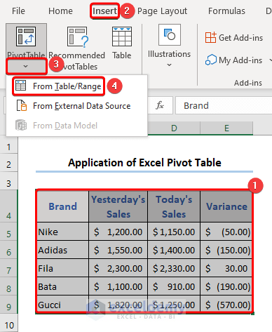
The sample dataset showcases the name of the Brand, and the present day, and the previous day sales.

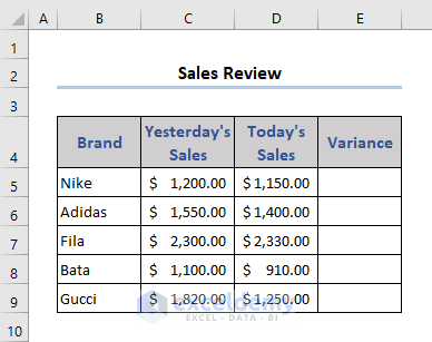
To find the variance of sales the following formula was used in E5. The Fill Handle icon was dragged down to the rest of the cells.

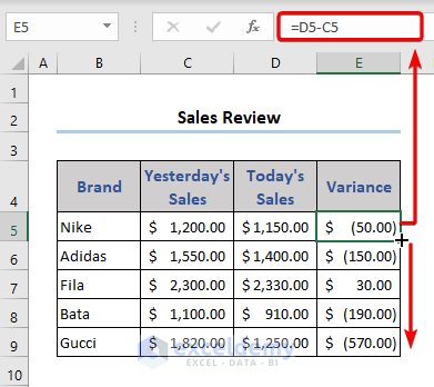
The output includes both positive and negative values in the Variance column.

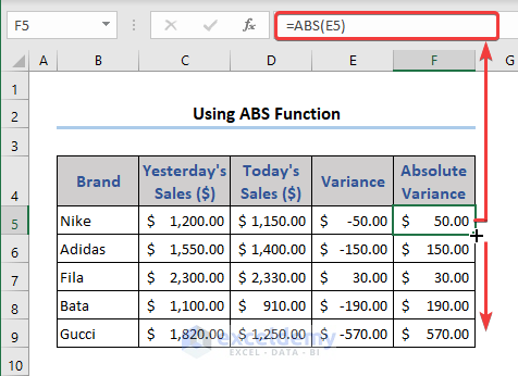
Method 1 – Using the Excel ABS Function to Get the Absolute Value

• Go to F5 and enter the following formula.

• Drag down the Fill Handle to see the result in the rest of the cells.

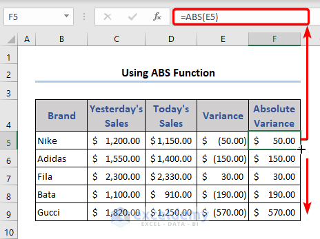
The ABS function returns the absolute value of the given reference.

Read More: Opposite of ABS Function in Excel

Method 2 – Apply a Condition Using the IF Function to the Get Absolute Value

• Go to F5 and enter the following formula.
• Drag down the Fill Handle to see the result in the rest of the cells.

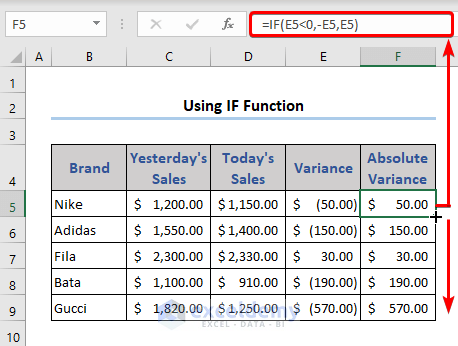
The absolute value for variances is displayed in column F.

Method 3 – Combining the SQRT and the POWER Functions to Find the Absolute Value

• Go to F5 and enter the following formula.
• Drag down the Fill Handle to see the result in the rest of the cells.

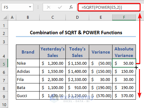
You can also use the caret (^)” operator instead of the POWER function:

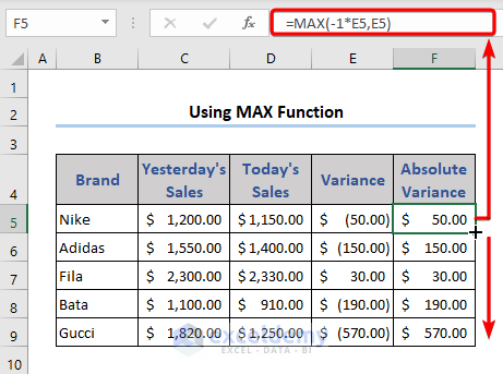
Method 4 – Using the Excel MAX Function to Get the Absolute Value by Comparing it to the Opposite Value

• Go to F5 and enter the following formula.
• Drag down the Fill Handle to see the result in the rest of the cells.

Method 5 – Using the SIGN Function to Multiply a Given Number by its Sign and get the Absolute Value

• Go to F5 and enter the following formula.

• Drag down the Fill Handle to see the result in the rest of the cells.

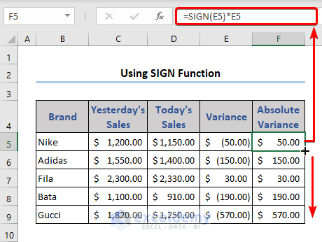
The formula converts the negative number into a positive, and the positive number does not change.

Method 6 – How to Get the Absolute Value Using a Pivot Table in Excel 

Steps:

• Select B4:E9 >> Insert >> PivotTable >> From Table/Range.

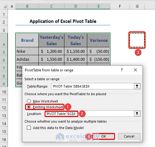
• In the PivotTable from table or range window, select Existing Worksheet.
• In Location, select G4.
• Click OK.

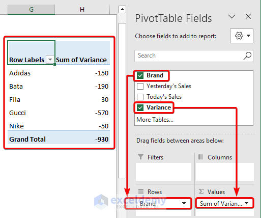
• PivotTable1 is created.

• Drag Brand into Rows and Variance into Values.

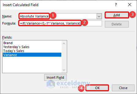
• Go to the PivotTable Analyze tab >> click Field, Items, & Sets  >> Calculated Field.

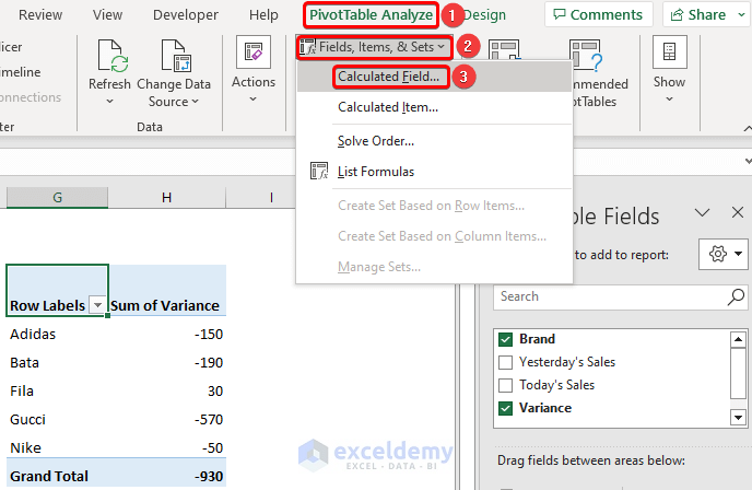
• In the Insert Calculated Field window, enter a name in Name and use the following formula in Formula.

• Click Add.
• Click OK.

This is the output.

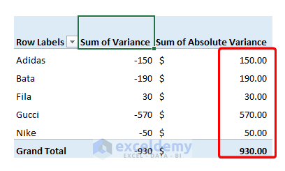
The absolute values of the Variance column are displayed in the Sum of Absolute Variance column.

Method 7 – How to Get the Absolute Value Using the Power Query in Excel

Steps:

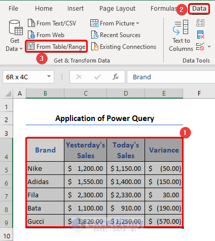
• Select B4:E9 >> go to Data >> From Table/Range.

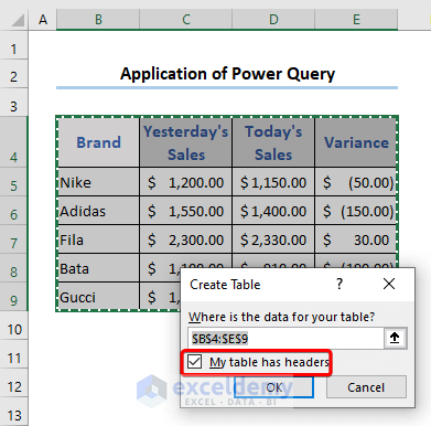
• In the Create Table window, check My table has headers.
• Click OK.

• In the Power Query Editor, select Add Column.
• Click Custom Column in General.

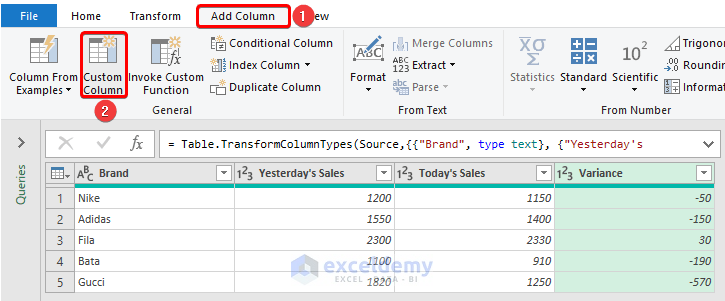
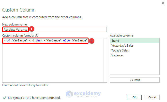
• Enter a name in New column name.
• Use the following formula in Custom column formula.

• Click OK.

This is the Power Query window:

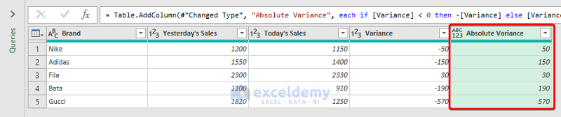
It displays the absolute values in the Absolute Variance column.

Method 8 –  Using a VBA Macro to Get the Absolute Values for a Large Excel Dataset

Steps:

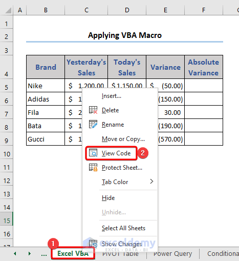
• Go to the Sheet Name and right-click.
• Choose View Code.

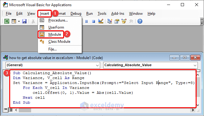
• In the VBA window, choose Module in the Insert tab.
• Enter the following VBA code in the Module.

Sub Calculating_Absolute_Value()
Dim Variance, V_cell As Range
Set Variance = Application.InputBox(Prompt:="Select Input Range", Type:=8)
    For Each V_cell In Variance
        V_cell.Offset(0, 1).Value = Abs(V_cell.Value)
    Next V_cell
End Sub

Code Breakdown

• Dim Variance, V_cell As Range

Declares two variables of the range type.

• Set Variance = Application.InputBox(Prompt:=”Select Input Range”, Type:=8)

Sets the value of Variance using an InputBox of the range type.

• For Each V_cell In Variance

              V_cell.Offset(0, 1).Value = Abs(V_cell.Value)

         Next V_cell

Applies a loop to each cell of Variance. The ABS function determines the absolute value for the V_cell and inserts that value into the next column of the same row. It moves to the next cell of V_cell.

• Run the VBA code by pressing F5.
• Select E5:E9 in Input.
• Click OK.

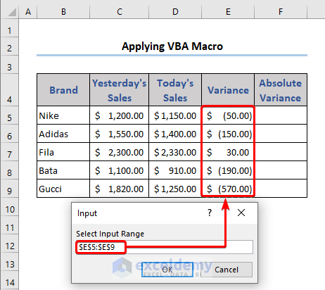
This is the output:

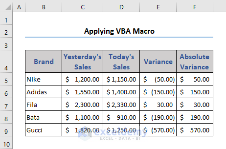
The absolute values are displayed in the Absolute Variance column.

How to Get the Absolute Value in Excel: 5 More Examples

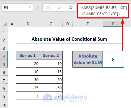
1. Calculate the Absolute Value of a Conditional Sum

The dataset contains two data series in columns B and C. To get the sum of values smaller than 0 in Series 1 and the sum of values greater than 0 in Series 2:

• Enter the formula in F4:

Formula Breakdown

• SUMIF(B5:B9,”<0″)

Determines the sum of values smaller than 0 in Series 1.

Result: -55

• SUMIF(C5:C9,”>0″)

Determines the sum of values greater than 0 in Series 2.

Result: 50

• ABS(SUMIF(B5:B9,”<0″)+SUMIF(C5:C9,”>0″))

determines the absolute value of the sum returned by the SUMIF functions.

Result: 5

Read More: Changing Negative Numbers to Positive in Excel

2. Calculate the Absolute Sum Value in an Array Formula

• Enter the following formula in E11 to get the absolute sum of the Variance array.

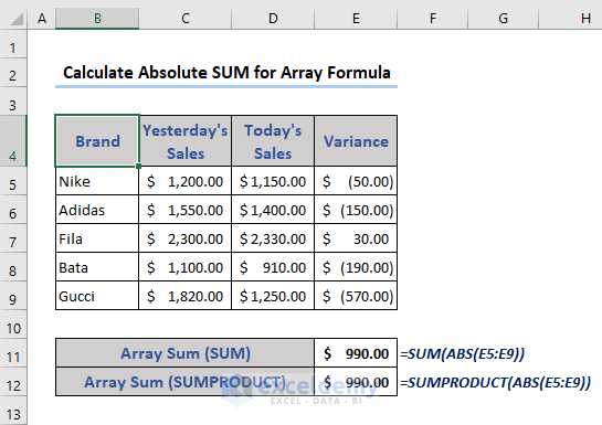
You can also use the formula below:

Read More: How to Sum Absolute Value in Excel

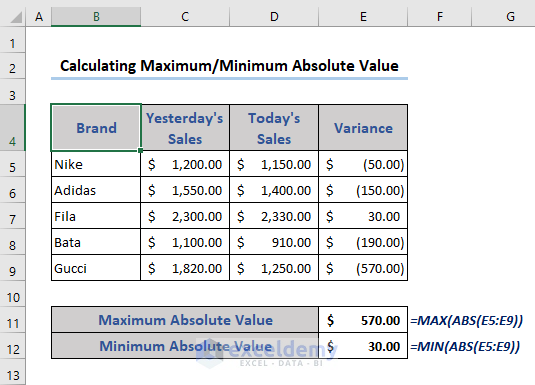
3. Find the Maximum/Minimum Absolute Value

• Enter the following formulas to get the maximum and minimum values in E11 and E12.

To get the maximum value:

To get the minimum value:

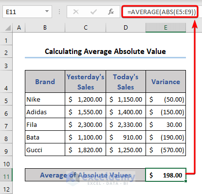
4. Calculate the Average of Absolute Values in Excel

• Use the formula in E11:

5. Calculate the Tolerance of the Variance

Steps:

• Find the tolerance of the variance using the following formula in F5.

• Drag down the Fill Handle to see the result in the rest of the cells.

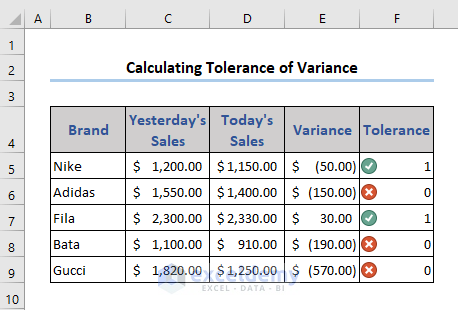
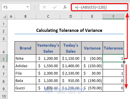If the variance is below the tolerance level 1 is displayed. Otherwise, 0.

• Select F5:F9 >> go to Conditional Formatting >> Icon Sets >> choose a symbol in Indicators.

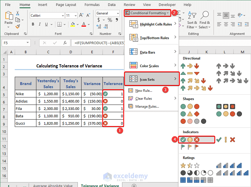
This is the output.

Read More: How to Calculate Absolute Difference between Two Numbers in Excel

Frequently Asked Questions

1. Can I get the absolute value of a complex number in Excel?

Ans: Yes, use the ABS function:  ABS(x).  x is the complex number.

2. Can I use the ABS function to calculate the distance between two numbers in a number line?

Ans: The distance between two numbers in a number line is the absolute value of the difference between two numbers. You can use the following formula: ABS(A1-A2).

Download Practice Workbook

Download the practice workbook.

Related Articles

• Calculate Absolute Percentage Error with Excel Function
• How to Make All Numbers Positive in Excel

<< Go Back to Excel ABS Function | Excel Functions | Learn Excel