If you want to apply a Filter based on text color this is the right place for you. Here, I will explain how to filter by text color in Excel. Sometimes from a large dataset based on criteria, you may need to Filter those values or text.
How to Filter by Text Color in Excel: 5 Methods
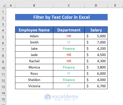
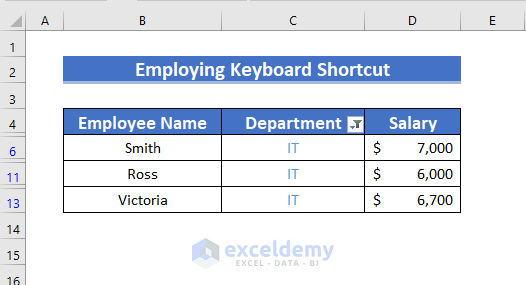
To clarify the explanation, I’m taking a sample Employee dataset along with their Name, Department, and Salary.
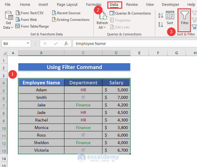
1. Using Filter Command to Filter by Text Color
You can use the Filter command to Filter by Text Color. A dataset may contain different types of text colors referring to different information.
- To begin with, select the data range where you want to apply the Filter.
- Here, I selected the cell range B4:D13.
- Next, open the Data tab >> select Filter.
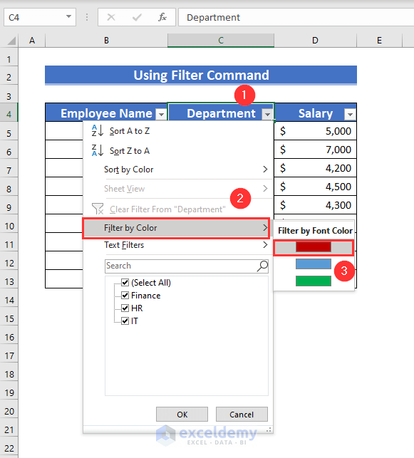
Now, the Filter Icon has appeared in the Column Header.
- First, click on the Filter Icon it will bring up a Context Menu.
- Then, from Filter by Color >> select the Filter by Font Color
- Here, I selected Red color.
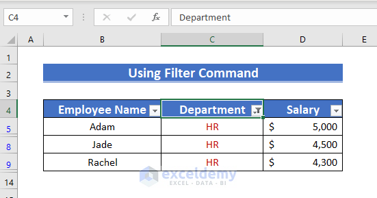
Therefore, you will get the Filtered result based on text color.
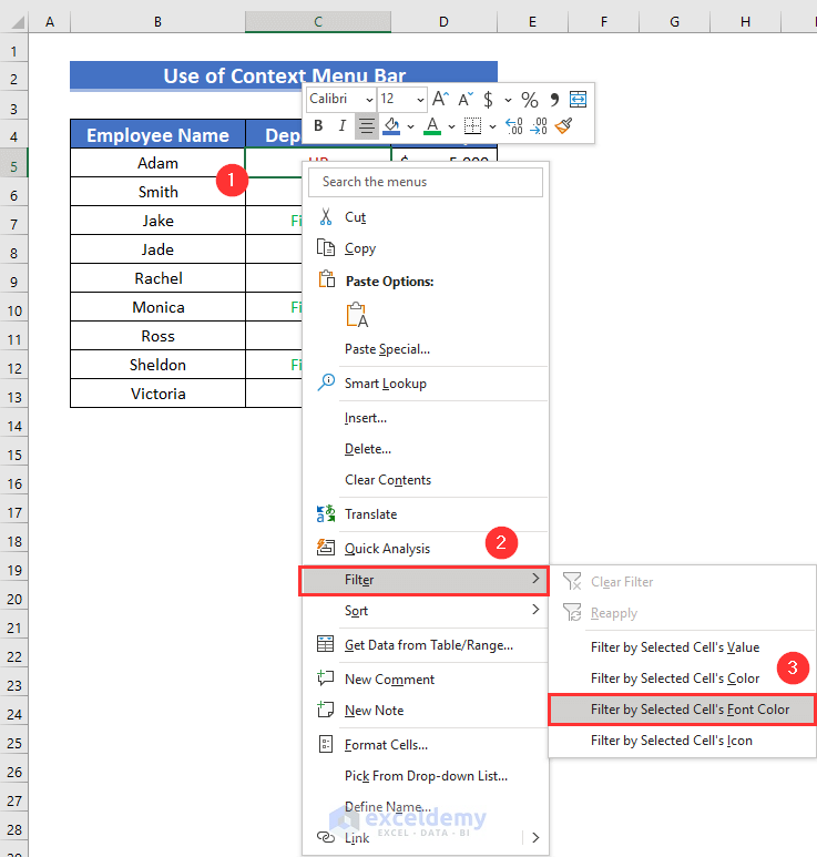
2. Employing Context Menu Bar in Excel
If you want, you can use the Context Menu Bar to Filter by Text Color. For that, you just need to select the particular text color for filtering.
- Firstly, select any text color of your choice. Here, I selected cell C5 which is Red color text.
- Secondly, right-click to bring up the Context Menu Bar.
- From there select Filter >> then choose Filter by Selected Cell’s Font color.
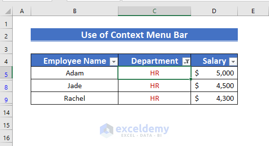
As a result, you will get the Filtered values by text color.
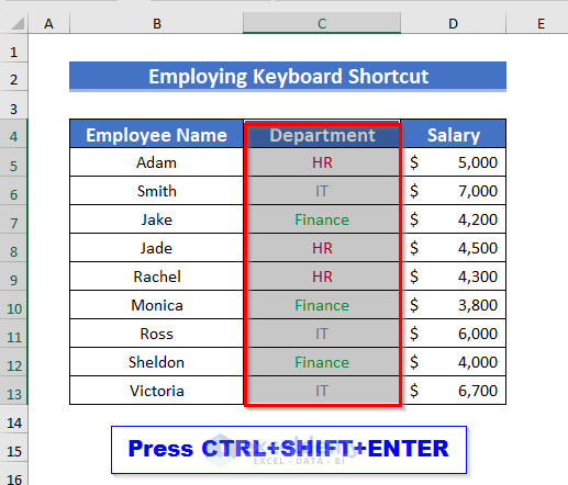
3. Using Keyboard Shortcuts in Excel
You also can use the Keyboard Shortcut to Filter by Text Color in Excel. It’s the easiest way to apply a filter.
- First, select any cell range to apply the Filter.
- Then, press CTRL+SHIFT+ENTER.
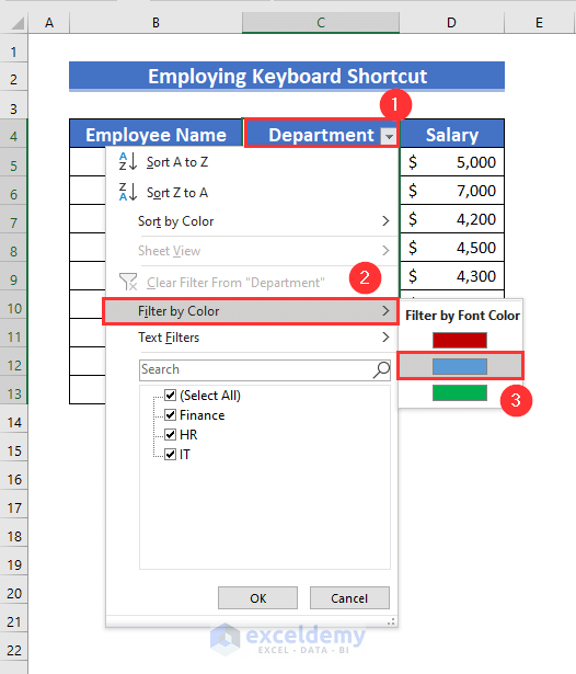
Now, the Filter icon will appear to filter by text color.
- First, click on the Filter Icon it will bring up a Context Menu.
- Then, from Filter by Color >> select the Filter by Font Color
- Here, I selected Blue color.
Now, you will get filtered values by text color.
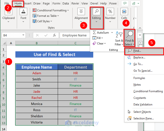
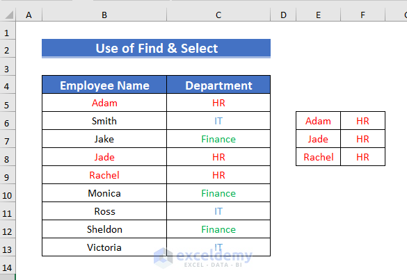
4. Using Find & Select Feature to Filter by Text Color in Excel
It is also possible to use the Find & Select feature to Filter by Text Color in Excel. But by following this method you can extract only the required result
- To begin with, select the data range from where you want to Find the text color to Filter.
- Here, I selected the cell range B4:C13.
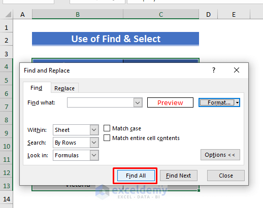
- Next, open the Home tab >> go to Editing >> from Find & Select >> select Find.
A dialog box of Find and Replace will appear.
- Next, select Format.
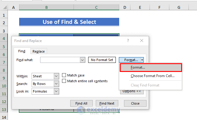
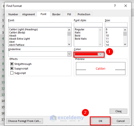
Another dialog box of Find Format will appear.
- Then, open the Font tab >> select Color (I selected Red)
- Next, click OK.
Now, you will be redirected to the Find and Replace dialog box.
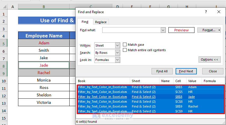
- Now, click on Find All.
Here, all the cells with Red color text will be available.
- Now, press CTRL+A to select all the findings.
- Then, close the dialog box.
- Now, press CTRL+C to copy the selected cells.
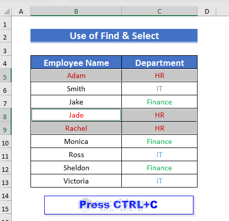
- Then, select any Empty cell to Paste the copied cells.
- Next, press CTRL+V to paste all the selected cells.
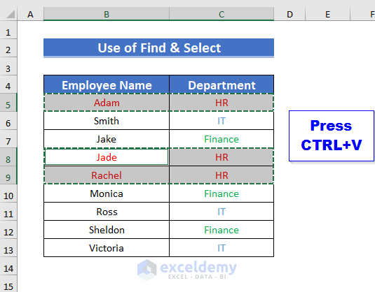
Moreover, values are Filtered by Text Color.
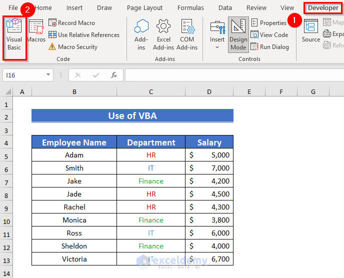
5. Use of VBA to Filter by Text Color in Excel
In case you want to use VBA the AutoFilter method is available for you to Filter by Text Color in Excel.
- Firstly, from the Developer tab >> select Visual Basic
You also can use the keyboard shortcut ALT+F11.
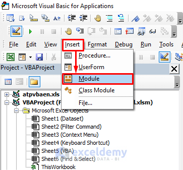
A window of VBA Editor will appear.
- Then, from Insert >> select Module.
- Type the following code in Module1.
Option Explicit
Sub Filter_by_Text_Color()

Worksheets("VBA").Range("B4:D13").AutoFilter Field:=2, _
   Criteria1:=RGB(192, 0, 0), Operator:=xlFilterFontColor

End Sub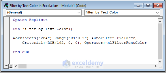
Code Breakdown
- First, I created a Sub procedure named Filter_by_Text_Color().
- Then used the Worksheets property to mention the sheet name VBA and used the Range property to mention the used range B4:D13.
- Next, I used the AutoFilter method where I used Field:=2 as I wanted to Filter Column 2.
- I want to filter the text containing the red color so I used RGB(192, 0, 0) as Criteria1.
- Finally, use Operator:=xlFilterFontColor so that the cells are filtered based on Font/Text color.
- Now, Save the code and go back to your worksheet.
- Open the Developer tab >> Select Macros.
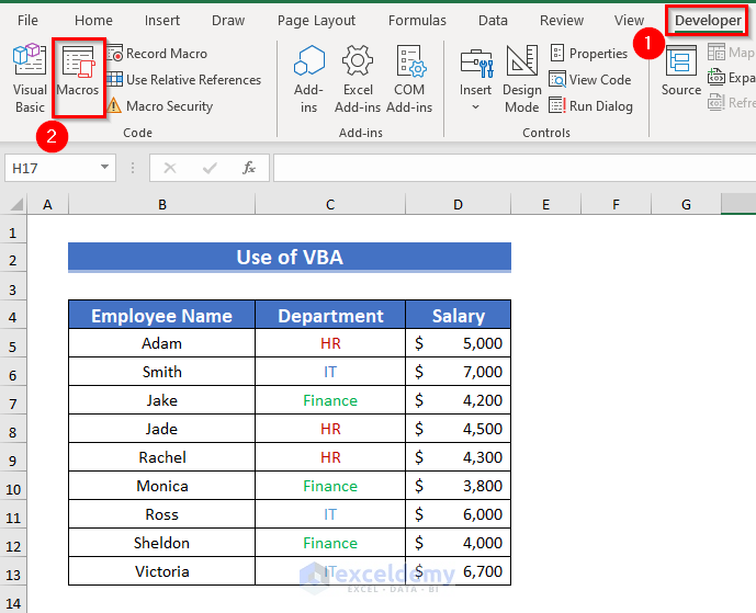
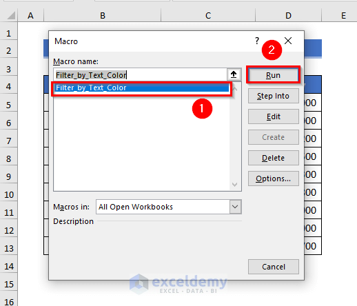
A dialog box of Macro will appear.
- Select the macro name Filter_by_Text_Color.
- Then, click on Run.
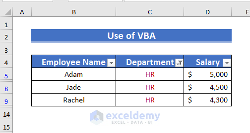
Therefore, you will get the Filtered values by Text Color.
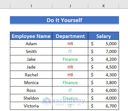
Practice Section
You can practice the explained methods here.
Download Practice Workbook
Conclusion
I tried to explain how to Filter by Text Color in Excel. This explanation will help you to understand the explained ways. Last but not least, if you have any kind of suggestions, ideas, or feedback please feel free to comment down below.
<< Go Back to Color Filter | Filter in Excel | Learn Excel
Get FREE Advanced Excel Exercises with Solutions!
