Today I’d like to introduce you to Excel’s OFFSET Function with 3 real-life examples.
At first, I will describe the formula syntax and then I’m going to talk about how the OFFSET function can be used to solve problems in real life.
Introduction
The OFFSET function can return a reference to a cell (let’s call it target cell) or range (target range) that is a specified number of rows and columns away from another cell (reference cell) or range (reference range).
The figure below illustrates how to use the OFFSET function to return the reference to a cell (left part) or a range (right part).
It will give you an intuitive impression of what is a target cell and what is a reference cell.
The cell highlighted in green is a target cell while cells highlighted in yellow consist of a target range.
Cells highlighted in blue are reference cells.
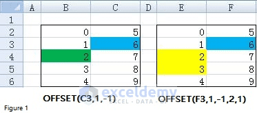
Figure 1
What does OFFSET mean in Excel (syntax)?
Here is the syntax of Offset Function: OFFSET (reference, rows, cols, [height], [width])
| Reference | Required. The reference is a cell or range of cells from which the offset begins. Please note that the cells must be adjacent to each other if you specify a range of cells. |
| Rows | Required. The number of rows, up or down, the reference cell or the upper-left cell of the reference range. Rows can be either positive or negative. Look at the left part of Figure 1, the target cell will be B2 if I change the function as OFFSET (C3, -1, -1). B2 is one row up C3. |
| Cols | Required. The number of columns, to the left or right, of the reference cell or the upper-left cell of the reference range. As with Rows argument, the values of Cols can also be both positive and negative. How can we write the OFFSET function if we set B4 as a reference cell and C3 as a target cell? The answer is OFFSET (B4, -1, 1). Here you can see that Cols is positive and C3 is one column to the right of B4. |
| Height | Optional. Only use the Height Argument If the target is a range. It tells how many rows that the target range includes. Height must be a positive number. You can see from the right part of Figure 1 that there are two rows in the target range. Therefore, we set Height as 2 in that case. |
| Width | Optional. Only use the Width Argument If the target is a range (see right part of Figure 1). It indicates how many columns that the target range contains. The width must be a positive number. |
Well, let me now show you how to use the OFFSET function to solve problems in real life.
Case 1: Right-to-Left Lookup by combining OFFSET and MATCH Functions
It’s well known that you can only perform a left-to-right lookup with the VLOOKUP function.
The value to search for must be placed in the first column of your table array.
You have to shift your entire table range to the right by one column if you want to add a new lookup value or you need to change your data structure if you’d like to use another column as the lookup value.
But by combining OFFSET together with the Match function, the limitation of the VLOOKUP function can be removed.
What’s the MATCH function and how can we combine the OFFSET function with the Match function to do the lookup?
Well, the Match function searches for a specified item in a range of cells and then returns the relative position of that item in the range.
Let’s take range B3:B8 from Figure 2.1 (which shows revenue of different countries in different years) as an example.
Formula “=MATCH (“USA”, B3:B8, 0)” will return 1 since USA is the first item in the range (see cell B10 and C10).
For another range C2:F2, the formula “=MATCH (2015, C2:F2, 0)” returns 3 as 2015 is the third item in the range (see cell B11 and C11).
Going back to the OFFSET function.
If we set cell B2 as the reference cell and take cell E3 as the target cell, how can we write the OFFSET formula?
E3 is 1 row below B2 and 3 columns right to B2.
Therefore, the formula can be written as “=OFFSET(B2, 1, 3)”. Look at the numbers in red color closely, can you find that they are matched?
That is the answer to the question – How to combine OFFSET function with Match function – Match function can be applied to serve as the second or the third argument of OFFSET function (see cell C13).
Cell C14 demonstrates how to use the VLOOKUP function to retrieve the same data.
We must know revenue in 2015 is recorded in the 4th column of the table array B2:F8 before writing the VLOOKUP function.
It means that we have to know very well about the data structure when using the VLOOKUP function.
This is another limitation for VLOOKUP. However, by using the MATCH function as the argument of the OFFSET function, we don’t have to know the column index.
This is very useful if there are lots of columns.
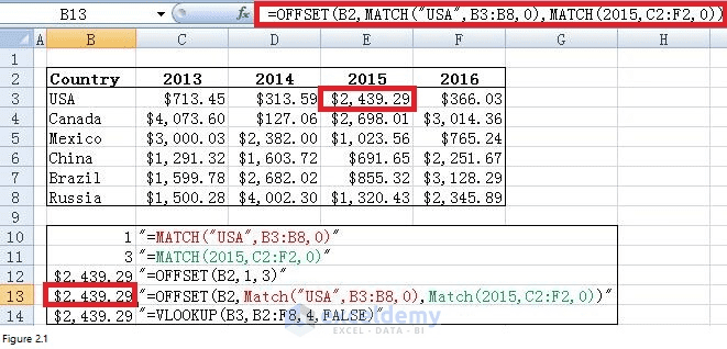
Figure 2.1
Now let’s move on and see a more complex example.
Suppose that we have a table containing Company Name, Contact Name, and Email Address for different companies.
And we want to retrieve the company name from a known contact name or get a contact name from a known email address. What can we do?
See Figure 2.2, range B5:E8 includes company information. By putting inputs in cell C2 and Cell B3, with the help of the formula in red square, I can retrieve the company name if I know the contact name.
Range D2:E4 shows how to get a contact name with a known email address.
In summary, these two examples illustrate that we can perform a right-to-left lookup and the search value does not need to be placed in the rightmost column. Any columns in the table array can contain the search value.
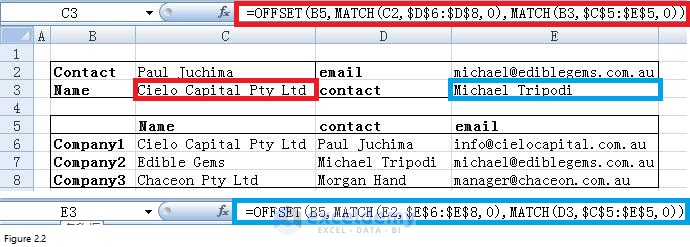
Figure 2.2
Case 2: Automate calculation combining OFFSET and COUNT functions
Before introducing on how to automate calculation whenever we add a new number in a column, let’s start with how to return the last number in a column automatically at first.
Look at the below figure which shows entries from Human Resources. Suppose that we want to get the last number in Column B, the formula would be “=OFFSET (C2, 9, 0)” if we apply the OFFSET function.
From the formula, we can know that 9 is the key number.
As long as we can return this number automatically, we can be able to locate the last number in a column automatically.
9 is just the number of cells that are containing numbers in column C.
If you are familiar with the COUNT function, you will know that the COUNT function can count the number of cells that contain numbers in a range.
For example, the formula “=COUNT (C3:C11)” will count the number of cells that contain numbers in cells C3 through C11.
In our case, we’d like to know how many numbers in a whole column, therefore, reference like C:C which includes all rows in column C should be used.
Please look at cells G4 and H4, the number returned by “=COUNT(C:C)” is exactly equal to 9.
Thus, by replacing 9 with COUNT(C:C) in the above OFFSET function, we can get a new formula “=OFFSET (C2, COUNT(C:C), 0)” (in cell H5).
The number it returns is 87000 which is exactly the last number in column C.
Now let move on to the automatic calculation. Suppose that we want the total of all the numbers in column C.
The formula would be “=SUM (OFFSET (C2, 1, 0, 9, 1))” if we use SUM together with OFFSET.
9 is the total number of rows in range C3:C11 and also the total number of cells contains numbers in column C.
Therefore, we can write the formula in a new way like “=SUM (OFFSET (C2,1, 0, COUNT (C:C), 1))”.
Look at cells G10 and H10, the total number of salaries for these 9 employees is $521,700.
Now if you put a number like $34,000 in cell C12, both the number in cell G5 and G10 will be changed to $34,000 and $555,700, respectively.
This is what I call automation as you don’t have to update formulas in cell G5 or G10.
You have to be careful when you use the COUNT function as the COUNT function only returns the number of cells that contain numbers.
For example, “=COUNT (B: B)” returns 0 instead 9 since there is no cell in column B that contains numbers (see cells G3 and H3).
Column D includes 10 cells containing numbers and the number returned by “COUNT (D: D)” is also 10.
But if we want to retrieve the last number in column D as we did for column C, we will get number 0 (see cell G8 and H8).
Obviously, 0 is not what we want. What’s wrong? Cell D13 is 11 rows away from cell D2 instead of 10 rows.
This also can be demonstrated by the formula “=OFFSET (D2, COUNT (D: D) + 1, 0)” in cell G7.
In summary, the numbers should be adjacent to each other if we want to use the COUNT function together with the OFFSET function to enable automation of calculation.
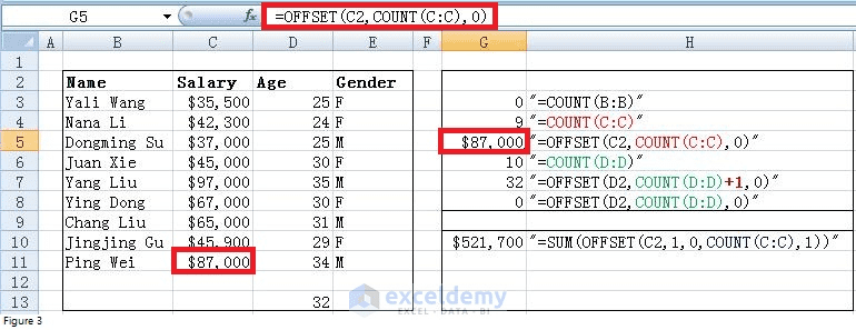
Figure 3
Case 3: Use OFFSET function to make a dynamic range
Suppose that we want to chart a company’s monthly unit sales and Figure 4.1 shows current data and a chart created based on current data.
Each month, the most recent month’s units’ sales will be added below the last number in column C.
Is there an easy way to update the chart automatically?
The key to updating the chart is to use OFFSET function to create dynamic range names for the Units Sold column.
The dynamic range for units’ sales will automatically include all sales data as new data is entered.
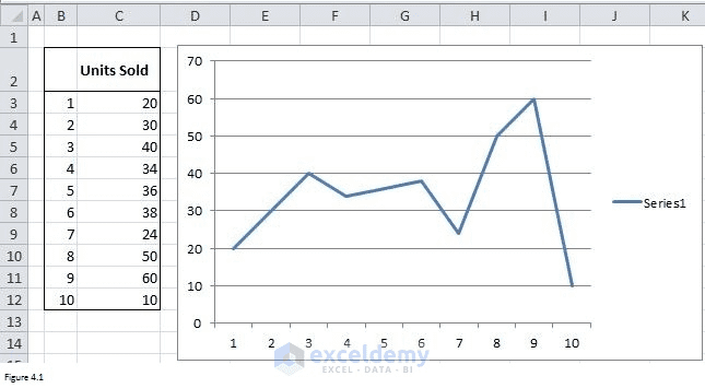
Figure 4.1
To create a dynamic range, click the Formulas tab and, then choose Name Manager or Define Name.
Below New Name dialog box will prompt if you click on Define Name.
If you choose Name manager, you also need to click on New to make the below New Name dialog box appear.
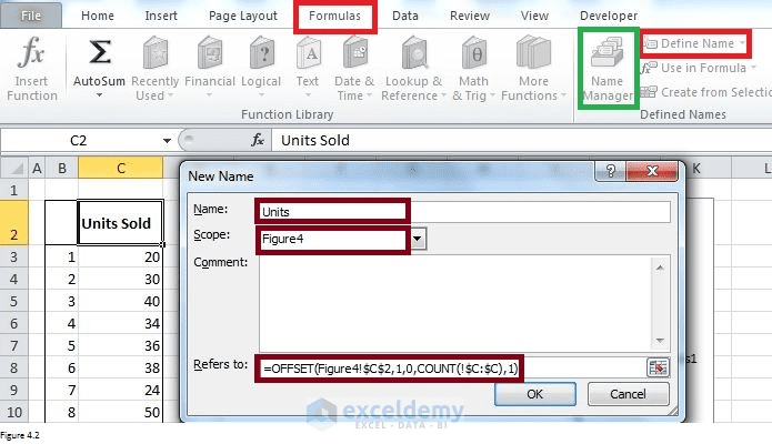
Figure 4.2
In the “Name:” input box, the dynamic range name should be filled in. And In the “Refers to:” input box, we need to type the OFFSET formula “=OFFSET (Figure4!$C$2, 1, 0, COUNT (!$C: $C), 1)” that would generate a dynamic range of values based on Units Sold values typed in column C.
By default, a name will apply to the whole workbook and must be unique within the workbook.
However, we want to restrict the scope to a particular sheet.
Therefore, we choose Figure4 here in the “Scope:” input box. After clicking on OK, the dynamic range is created.
It will automatically include all sales data as new data is entered.
Now right-click on any point in the chart and then select “Select Data”.
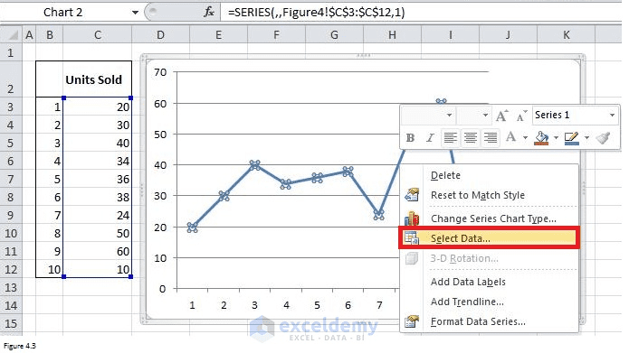
Figure 4.3
In the prompted Select Data Source, choose Series1 and then Edit.
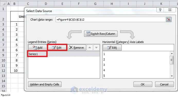
Figure 4.4
And then type “=Figure4!Units” as Figure 4.5 shows.
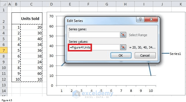
Figure 4.5
Finally, let’s have a try and type 11 in cell C13. You can see the chart has changed and value 11 has been included.
The chart will change automatically when new data is added.
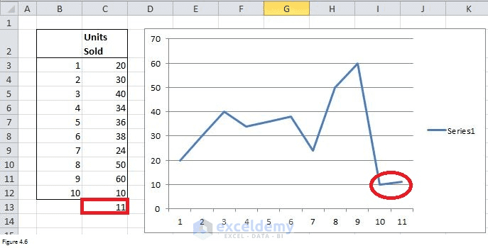
Figure 4.6
Read More…
Download working files
Download the working files from the link below.
Get FREE Advanced Excel Exercises with Solutions!
