How to Set Floating Picture in Excel (with Easy Steps)

In this article, I will show how to set a floating picture in Excel. In many situations, we need to keep a picture side by side when scrolling through the Excel worksheet. For example, there are many situations when we need to compare a long vertical list of data with a picture. Here I will discuss how to deal with this kind of situation. So let’s get started.

Download Practice Workbook

Download this practice workbook to exercise while you are reading this article.

Step-by-Step Procedure to Set Floating Picture in Excel

 Before going to set up the Excel floating picture, let’s take a sample worksheet to contextualize the problem first. In the picture below, I have taken a worksheet where there is some information about 50 students of a College. The information includes Name, Student ID, Gender, and Blood Group. On the right side of the data table, we have a picture of the Blood Type Compatibility Table.

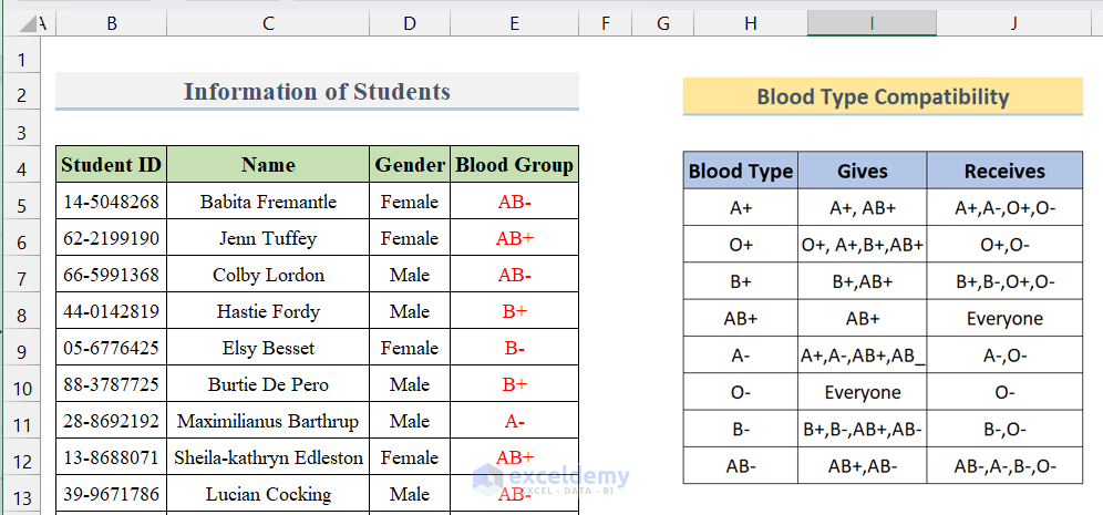
As we scroll down below, we want that the picture of the Blood Type Compatibility table floats with us so that we can easily check whether a student is able to donate or receives a certain group of blood. For example, even when we reach the bottom of the table, we want the picture to appear there at the top right corner of the screen. So how do we do that? To know, follow the steps below.

Step-1: Opening Private Module in VBA

First, we need to open a private module in Visual Basic Window. To do that, follow the steps below.

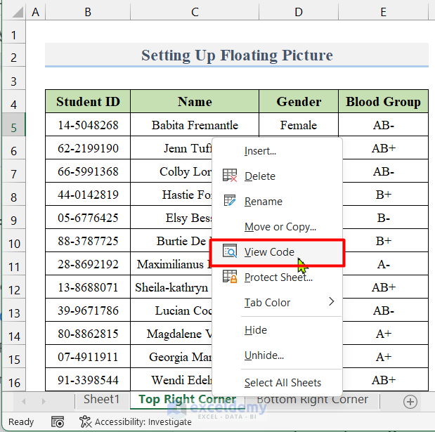
• We first need to open the Microsoft Visual Basic Window. To do that, bring your mouse cursor to the bottom of the screen on the top of the name of the worksheet and then right-click on it. After that, select the View Code.

• As a result, the Microsoft Visual Basic Window will open up.

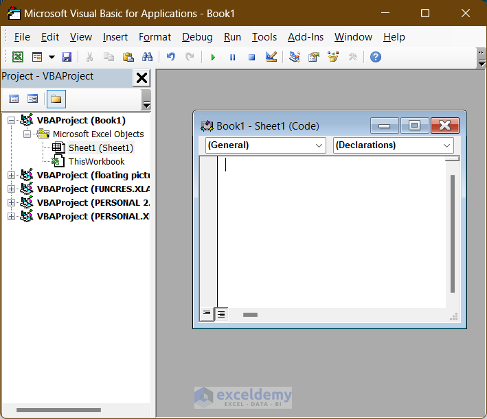
• Alternatively, you can also type Alt+F11 to open the editor and then double-click on the sheet.

Step-2: Writing VBA Code in Private Module

In the 2nd step, we will write a code in the Module. Follow the steps below.

• Now, copy-paste the code below in the window.

'Right Right Corner
Private Sub Worksheet_SelectionChange(ByVal A_Target As Excel.Range)
    Dim My_Picture As Object
    Dim My_Top As Double
    Dim My_Right As Double
    Dim Top_Right_Cell As Range
    '-----------------------------------------------------------
    '- position of the bottom right cell
    With ActiveWindow.VisibleRange
        AA_r = 1
        AA_c = .Columns.Count
        Set Top_Right_Cell = .Cells(AA_r, AA_c)
    End With
    '------------------------------------------------------------
    '- Setting position of the picture
    Set My_Picture = ActiveSheet.Pictures(1)
    My_Top = Top_Right_Cell.Top + 5
    My_Right = Top_Right_Cell.Left - My_Picture.Width - 5
    With My_Picture
        .Top = My_Top
        .Left = My_Right
    End With
End Sub

• Now, close the window and return to the Worksheet.

Read More: How to Create Floating Cells in Excel (2 Easy Methods)

Step-3: Scrolling Down in Worksheet

In the final step, we will check whether our code is working properly or not by scrolling through the worksheet.

• Now, if we scroll down below, the moment we click on any cell, the floating picture will appear on the top right corner of the window.

• If you want your floating picture to be on the bottom right corner of the window, you have to copy and paste the following code on the developer window.

   'Bottom Right Corner
Private Sub Worksheet_SelectionChange(ByVal A_Target As Excel.Range)
    Dim My_Picture As Object
    Dim My_Top As Double
    Dim My_Left As Double
    Dim Bottom_Right_Cell As Range
    '-----------------------------------------------------------
    '- position of the bottom right cell
    With ActiveWindow.VisibleRange
        AA_r = .Rows.Count
        AA_c = .Columns.Count
        Set Bottom_Right_Cell = .Cells(AA_r, AA_c)
    End With
    '------------------------------------------------------------
    '- Setting position of the picture
    Set My_Picture = ActiveSheet.Pictures(1)
    My_Top = Bottom_Right_Cell.Top - My_Picture.Height - 5
    My_Left = Bottom_Right_Cell.Left - My_Picture.Width - 5
    With My_Picture
        .Top = My_Top
        .Left = My_Left
    End With
End Sub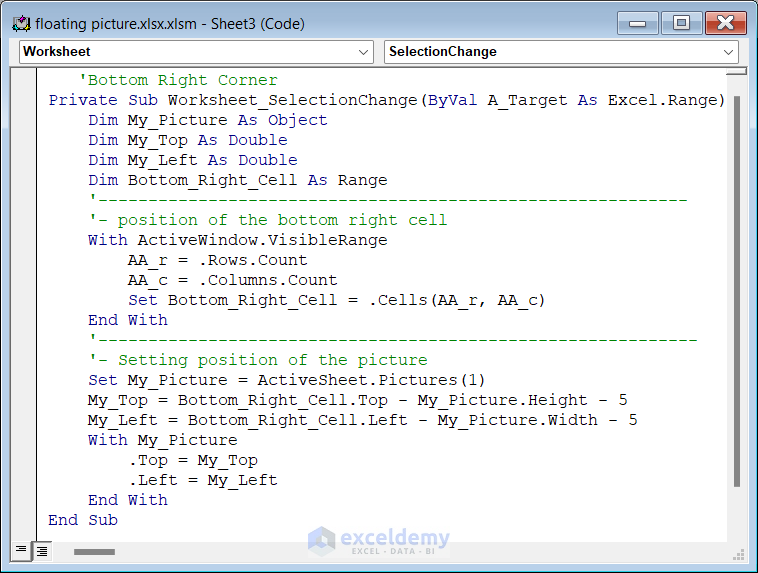

• Now, if you scroll down and click any cell, the floating picture will appear on the bottom right corner of the window.

This is how easily we can have a floating picture in an Excel worksheet that can move with the visible window.

Floating Box Visible While Scrolling in Excel

In this section, I will show you how to make a floating box visible while scrolling in Excel. Taking the previous example given above, this time we will try to make a floating box appear instead of a floating image. Here, we will show a box that will contain the number of students who has O +ve as blood group.

To do that, follow the steps below.

Steps:

• First, let’s have a cell(G5) where we have calculated the number of students who have O+ as blood group using the following formula.

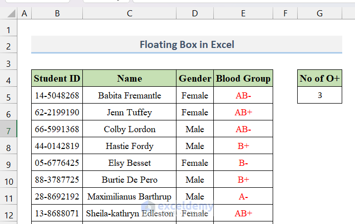
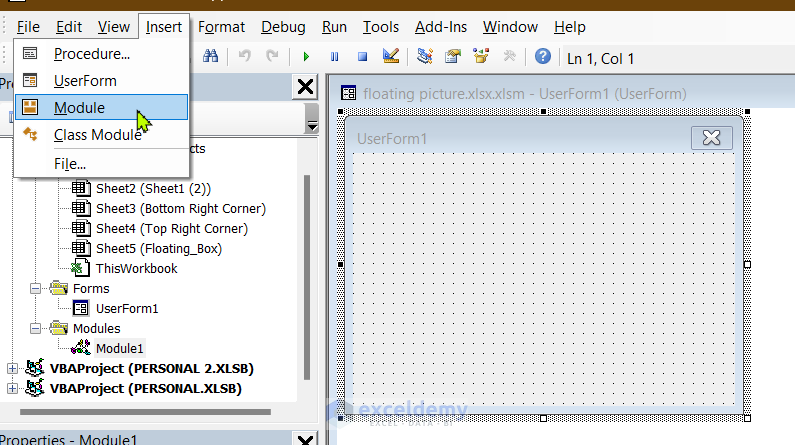
• Now, we will create a box that will contain the data of cell G5 and make the box float as we scroll. To do that, open the VBA editor by clicking Alt+F11. Then go to Insert> Userform.

• As a result, a Userform will be created like this.

• Now, insert a module by going to Insert > Module.

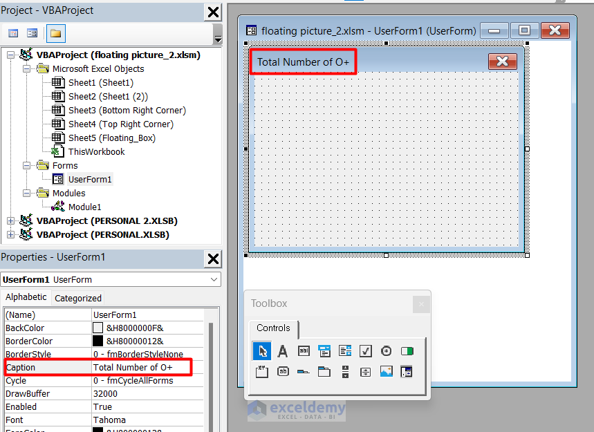
• Now, go back to the created UserForm1 by double-clicking on the menu bar located on the left side.

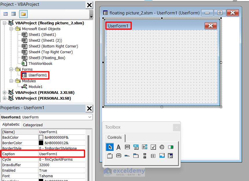
• Here in the bottom corner, you should see the properties of UserForm 1. If you don’t see the properties tab, you can right-click on the user form window and then select properties. Now, edit the caption and give it a suitable one. I am giving it Total Number of O+.

• Now, as the userform is empty, we can insert a text box or a label. I amtaking a label named Label1. To do that, click on the A icon from the Controls in the Toolbox and draw a box on the user form window.

• Now, right-click on the user from the window and select view code. Consequently, the Code window will open up.

• Now, choose Initialize from the dropdown menu. (see the screenshot below)

• Now,write down the following code and clear the above portion.

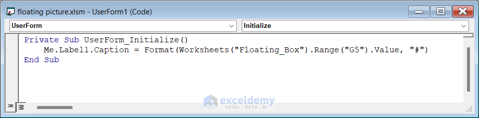
Private Sub UserForm_Initialize()
    Me.Label1.Caption = Format(Worksheets("Floating_Box").Range("G5").Value, "#")
End Sub

• Now, click on the worksheet to open the code of that sheet. Then from the left and right dropdown menu, choose Worksheet and Calculate.

• Now, copy-paste the following code.

Private Sub Worksheet_Calculate()
UserForm1.Label1.Caption = Format(Worksheets("Floating_Box").Range("G5").Value, "#")
End Sub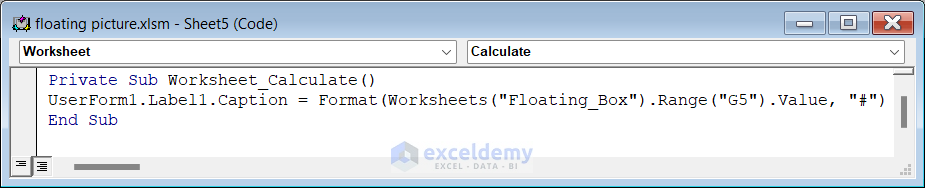

• Now, we will write a code in Module1 to open a Macro. To do that, go to Module by clicking on the Module1 and write the following code.

Sub ShowForm()
UserForm1.Show False
End Sub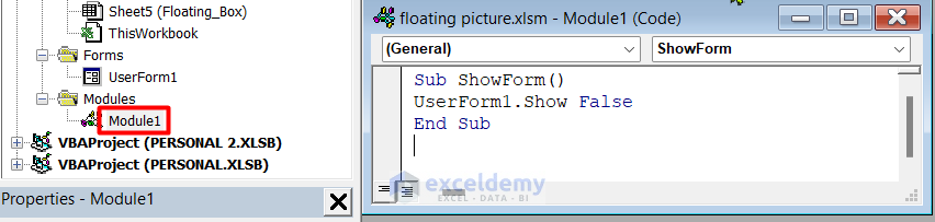

• Now, go to the worksheet and then press Alt+F8 to open the macro list. Then select the ShowForm macro and run it.

• As a result, you will see that the form will appear on the worksheet containing the total number of O+. And even if we scroll through the worksheet, the form will still float.

• Now, if we change O+ to something else, it will immediately reflect on the floating form.

Read More: How to Insert Floating Table in Excel (2 Easy Ways)

Things to Remember

• The floating picture will only appear after you click on a cell while scrolling.
• After writing the given code, you can not use the Undo command(Ctrl+Z) . This is a major con of this code.

Conclusion

That is the end of this article regarding how we can set a floating picture in Excel. If you find this article helpful, please share this with your friends. Moreover, do let us know if you have any further queries. Finally, please visit Exeldemy for more exciting articles on Excel.

Related Articles

• How to Add Floating Comment in Excel (3 Simple Methods)
• Remove Floating Cells in Excel (3 Easy Ways)