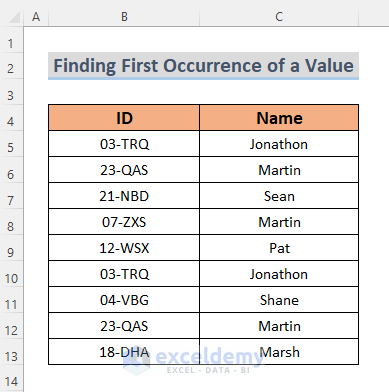
We are using a dataset that contains IDs and Names of some guys. The dataset contains some duplicates, so we’ll find only the first occurrence of particular values.
How to Find the First Occurrence of a Value in a Column in Excel: 5 Ways
Method 1 – Using the Excel COUNTIF Function to Find the First Occurrence of a Value in a Column
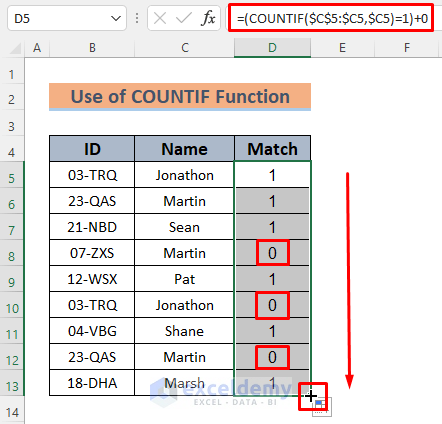
If any name occurs twice or more in this dataset, we will mark them with 0. Otherwise, it will be marked as 1.
Steps:
- Make a new column D to identify the occurrences and use the following formula in cell D5.
=(COUNTIF($C$5:$C5,$C5)=1)+0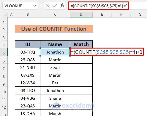
Here, the COUNTIF function keeps returning TRUE until it finds the same name in the column C. We added a 0 (zero) to get the numerical value.
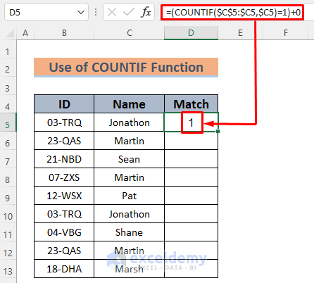
- Hit Enter and you will see the output in cell D5.
- Use the Fill Handle to AutoFill the other cells.
Method 2 – Applying the COUNTIFS Function to Find the First Occurrence of a Value in a Column
If any name occurs twice or more in this dataset, we will mark them as 0. Otherwise, we’ll mark them as 1.
Steps:
- Make a new column D to identify the occurrences and use the following formula in cell D5.
=N(COUNTIFS(C$5:C5,C5)=1)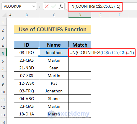
Here, the COUNTIFS function keeps returning TRUE until it finds the same name in the column C. The N function converts TRUE or FALSE to 1 or 0 respectively.
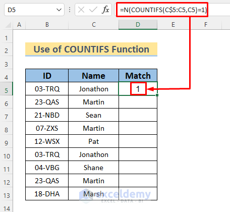
- Hit Enter and you will see the output in cell D5.
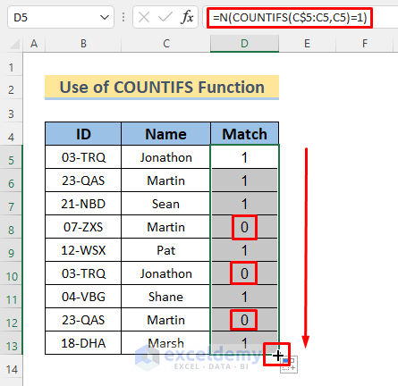
- Use the Fill Handle to AutoFill the other cells.
Method 3 – Find the First Occurrence of a Value in a Column by Utilizing the Excel ISNUMBER and MATCH Functions
If any name occurs twice or more in this dataset, we will mark them with a 0. Otherwise, we mark them with a 1.
Steps:
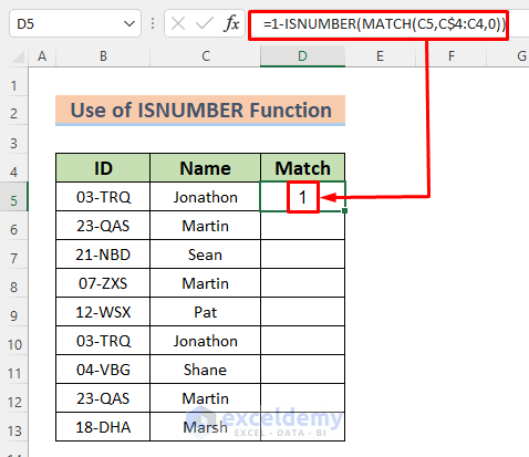
- Make a new column D to identify the occurrences and use the following formula in cell D5.
=1-ISNUMBER(MATCH(C5,C$4:C4,0))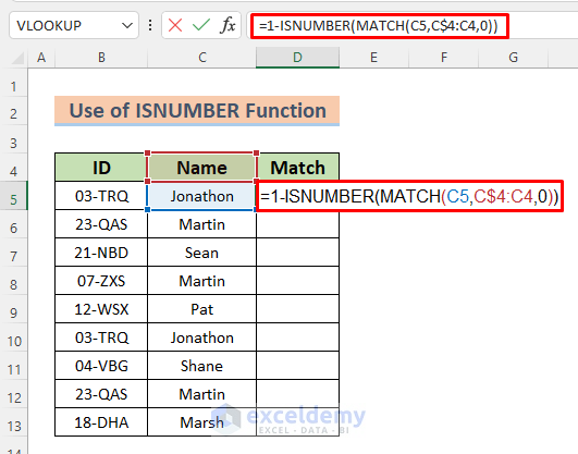
Here, the MATCH function searches for the value in C5, looks up through the range C4:C4 and returns the position where it finds an exact match. The ISNUMBER function returns TRUE if it finds a numeric value in it. Otherwise, it returns FALSE even if it has an error in it.
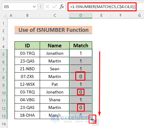
- Press the Enter button and you will see the output in cell D5.
- Use the Fill Handle to AutoFill the column.
Read More: How to Find First Occurrence of a Value in a Range in Excel
Method 4 – Finding the First Occurrence of a Value by Using Combined Functions
If any ID occurs twice or more in this dataset, we will mark them with 0. Otherwise, we mark them with a 1.
Steps:
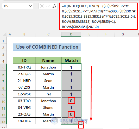
- Make a new column D to identify the occurrences and use the following formula in cell D5.
=IF(INDEX(FREQUENCY(IF($B$5:$B$13&"#"&$C$5:$C$13<>"",MATCH("~"&$B$5:$B$13&"#"&$C$5:$C$13,$B$5:$B$13&"#"&$C$5:$C$13,0)),ROW($B$5:$B$13)-ROW($B$5)+1),ROWS($B$5:B5))>0,1,0)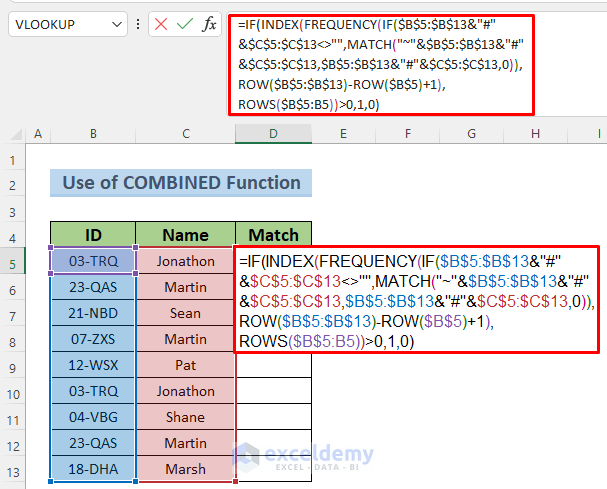
Here, the IF function returns 1 (TRUE) when it meets the criteria, else it returns 0 (FALSE). The FREQUENCY function determines the number of times a value occurs within a given range of values.
Formula Breakdown
- ROWS($B$5:B5) —-> Returns
- Output: 1
- ROW($B$5:$B$13) —-> Becomes
- Output: {5;6;7;8;9;10;11;12;13}
- ROW($B$5) —-> Turns into
- Output: {5}
- MATCH(“~”&$B$5:$B$13&”#”&$C$5:$C$13,$B$5:$B$13&”#”&$C$5:$C$13,0) —-> Becomes
- Output: {1;2;3;4;5;1;7;2;9}
- IF($B$5:$B$13&”#”&$C$5:$C$13<>””,MATCH(“~”&$B$5:$B$13&”#”&$C$5:$C$13,$B$5:$B$13&”#”&$C$5:$C$13,0)) —-> Turns into
- IF($B$5:$B$13&”#”&$C$5:$C$13<>””,{1;2;3;4;5;1;7;2;9}) —-> leaves
- Output: {1;2;3;4;5;1;7;2;9}
- FREQUENCY(IF($B$5:$B$13&”#”&$C$5:$C$13<>””,MATCH(“~”&$B$5:$B$13&”#”&$C$5:$C$13,$B$5:$B$13&”#”&$C$5:$C$13,0)),ROW($B$5:$B$13)-ROW($B$5)+1) —-> Becomes
- FREQUENCY(IF{1;2;3;4;5;1;7;2;9}),{5;6;7;8;9;10;11;12;13}-{5}+1) —-> Turns into
- Output: {2;2;1;1;1;0;1;0;1;0}
- INDEX(FREQUENCY(IF($B$5:$B$13&”#”&$C$5:$C$13<>””,MATCH(“~”&$B$5:$B$13&”#”&$C$5:$C$13,$B$5:$B$13&”#”&$C$5:$C$13,0)),ROW($B$5:$B$13)-ROW($B$5)+1) —-> Returns
- INDEX({2;2;1;1;1;0;1;0;1;0})
- Output: {2}
- IF(INDEX(FREQUENCY(IF($B$5:$B$13&”#”&$C$5:$C$13<>””,MATCH(“~”&$B$5:$B$13&”#”&$C$5:$C$13,$B$5:$B$13&”#”&$C$5:$C$13,0)),ROW($B$5:$B$13)-ROW($B$5)+1),ROWS($B$5:B5))>0,1,0) —-> Simplifies to
- IF({2}>0,1,0)
- Output: 1
We get the output as 1 because the ID in cell B5 occurs for the first time.
- Hit Enter, and you will see the output in cell D5.
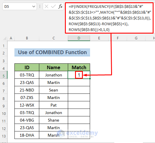
- Use the Fill Handle to AutoFill the other cells.
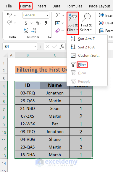
Method 5 – Using the Filter Command to Sort First Occurrences of Values in a Column
Suppose you want to see the repeat times of the names in column D and hence you want to see the position of the first occurrences of these names.
Steps:
- Make a new column D to identify the occurrences and use the following formula in cell D5.
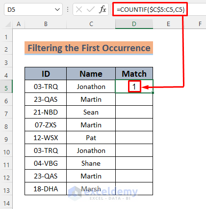
=COUNTIF($C$5:C5,C5)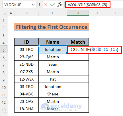
Here, the COUNTIF function returns the number of times a name occurs in column C up to that cell.
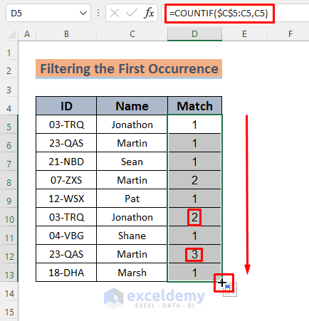
- Hit Enter.
- Use the Fill Handle to AutoFill the column.
- To Filter the first occurrences, select the range B4:D13 and go to Home, choose Sort & Filter, and select Filter
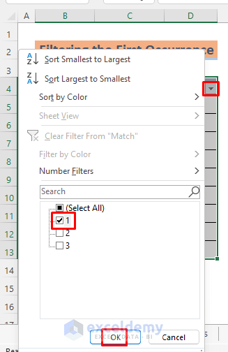
- Click on the marked arrow in the Match header.
- Mark 1 and click OK.
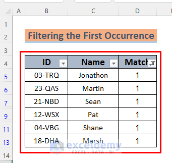
- You will see all the duplicate IDs hidden by the filtering.
Read More: How to Find Last Occurrence of a Value in a Column in Excel
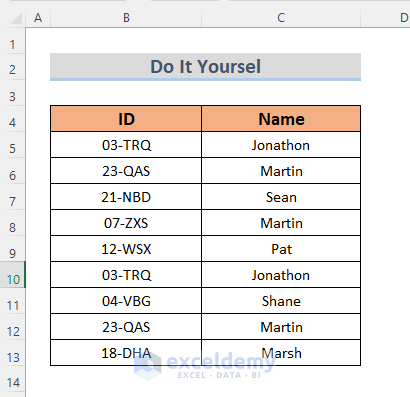
Practice Section
Here’s the dataset we used in this article which you can use to practice these methods on your own.
Download the Practice Workbook
Related Articles
- How to Find Multiple Values in Excel
- How to Find First Value Greater Than in Excel
- Find Last Value in Column Greater than Zero in Excel
- How to Find Value in Column in Excel
<< Go Back to Find Value in Range | Excel Range | Learn Excel
Get FREE Advanced Excel Exercises with Solutions!

Just wanted to thank you for a simple solution to a problem I was having. Was able to add one of your suggestions to an already complex formula and fix my issue the first time. Thank you for your effort to create articles of this type.
Hey Pam, it’s really nice to see you get benefit from my article. It’s also an honor because I work with sincerity for these articles so the readers can have their solutions in the easiest way possible. I appreciate your compliment and also hope that my other articles can be useful for you as well. You are welcome!!!
Hello Nahian,
Thanks for the solution!
Is there a way to modify the combined formula to check for the last occurrence of a value in a column?
I have slightly modified your first occurrence formula to check only one column. Placing a “PO” where the first occurrence of a value in the column.
=IF(INDEX(FREQUENCY(IF($B$4:$B$500″”,MATCH($B$4:$B$500,$B$4:$B$500,0),0),ROW($B$4:$B$500)-ROW($B$4)+1),ROWS($B$4:B4))>0,”PO”,””)
Hi Jason, thanks for reaching out. I’ve used your formula and it returns PO for some values. However, I think I have a better idea for your solution.
Here, I made a drop down list using the names of the dataset (C5:C13 range). My target is, whenever you select a name, Excel will highlight the cell where the name last appeared.
Here is the drop down list.
And here is the formula with XLOOKUP and ROW functions to determine the row of last appearance of the name selected from the drop down list.
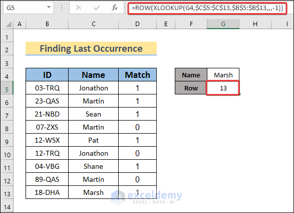
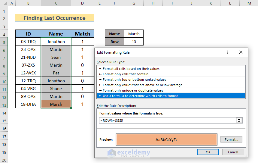
=ROW(XLOOKUP(G4,$C$5:$C$13,$B$5:$B$13,,,-1))To highlight the cell with the last occurrence, we need to set a formula for conditional formatting. So select the range of names (C5:C13) and then go to Home >> Conditional Formatting >> New Rule >> Use a formula to determine which cells to format and insert the formula below.
 Click the image to get a detailed view.[/caption]
=ROW()=$G$5[caption id="attachment_427897" align="aligncenter" width="750"]
After that, choose a fill color to format the cell and click OK.
Finally, if you select any name from the drop down, you will see the cell highlighted where the name occurred for the last time in column C.
Here, we selected Martin from the drop down and you can see that the name Martin appears 3 times in column C. But only the C12 cell is highlighted as it is the last time the name Martin appeared.
Figured it out! Thanks again Meraz!
=IF(ROW(A4)=(ROW(XLOOKUP(B4,$B$4:$B$15,$B$4:$B$15,,,-1))),”PI”,””)
Thanks for the quick feedback!
Xlookup is great for identifying the row in which the last value appears. Based on the application in which I am trying to use it, it’s only one piece of the puzzle (and I can’t figure out where to fit the piece in your original combined formula).
Looking at the sheet below, I am trying to flag “PI” in column A where the last value appears in column B.
Row A B
1 1
2 1
3 PI 2
4 3
5 4
6 PI 1
7 5
8 PI 5
9 PI 3
10 PI 4
Dear Jason,
You are most welcome.
Regards
ExcelDemy