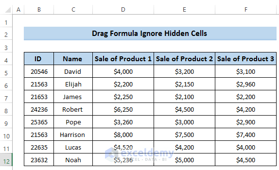
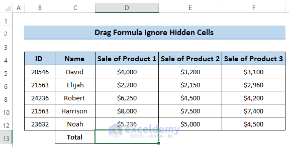
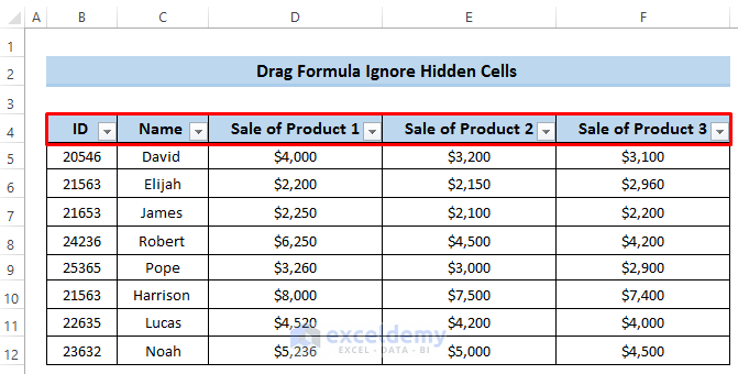
This is the sample dataset.
Example 1 – Drag Formula and Ignore Hidden Cells Using SUBTOTAL Function
Steps
- Press Ctrl and select row 7, row 9, and row 11.
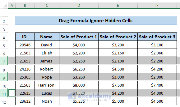
- Right-click on the selected rows.
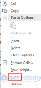
- A Context Menu will appear.
- Select Hide.
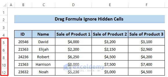
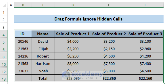
- It will hide all the selected rows. See the image below.
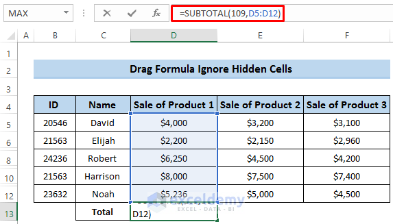
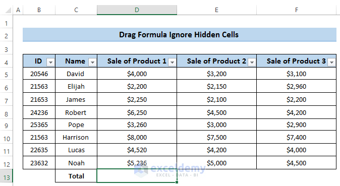
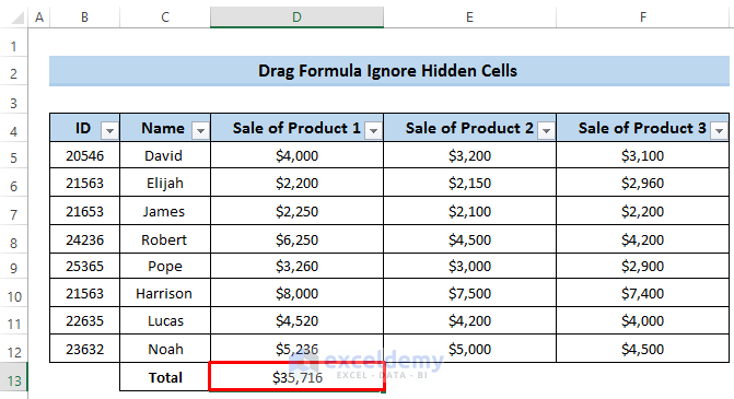
- To find out the total income from product 1 sale, use the SUBTOTAL function.
- Select cell D13.
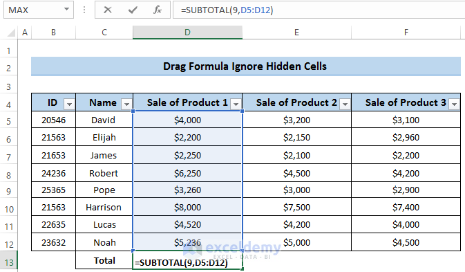
- Enter the following formula.
=SUBTOTAL(109,E5:E12)109 is the function_num which denotes the SUM function but will ignore hidden cells while applying.
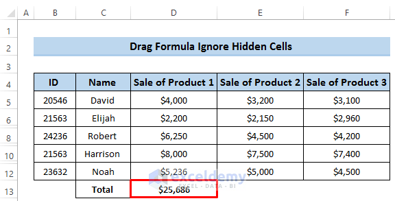
- Press Enter to apply the formula.
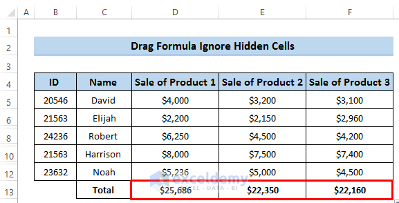
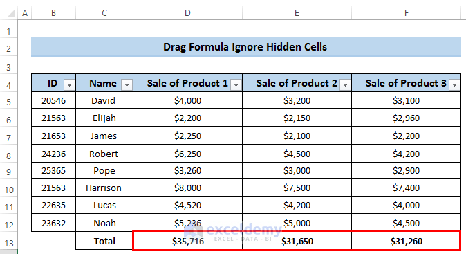
- Drag the Fill Handle icon to the right to fill down the next value. It will calculate the sum of product 2 and product 3. In all the cases, the function ignores the hidden cells.
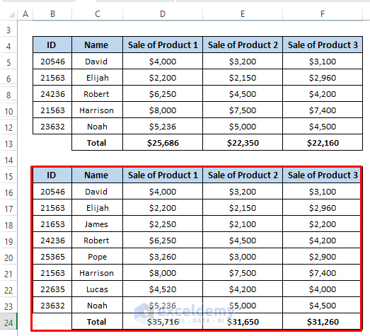
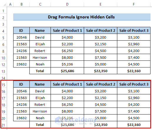
- Copy the range of cell B4 to F13.
- Select B15 and paste it. All the hidden cells will be displayed with the updated sum value.
- Drag the formula ignoring hidden cells.
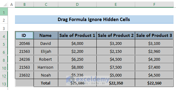
- Select the range of cells B4 to F13.
- Press ‘Alt+;’. See the image below.
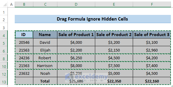
- Press Ctrl+C to copy the selected range of cells. It will highlight the cells as shown in the image below.
- Select cell B15.
- Paste the selected range of cells.
- The cells and formula ignores the hidden cells.
Note:
You can’t paste the selected range of cells with some hidden cells on the right side of the original dataset. You can paste it either below the dataset or into another worksheet. This is because you hide some cells in the dataset so if you paste it on the right side of the dataset, the paste value must use the same rows as the original dataset.
Read More: How to Drag Formula in Excel with Keyboard
Example 2 – Drag Formula and Ignore Hidden Cells Using AGGREGATE Function
Steps
- Press Ctrl and select row 7, row 9 and row 11.
- Right-click on the selected rows.
- A Context Menu will appear.
- Select Hide.
- It will hide all the selected rows.
- To find out the total income from product 1 sale, use the SUBTOTAL function.
- Select cell D13.
- Enter the following formula.
=AGGREGATE(9,5,D5:D12)9 is the function_num which denotes the SUM function. Next, we will get some more options. Where 5 denotes ignore hidden rows.
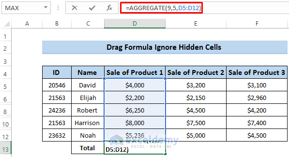
- Press Enter to apply the formula.
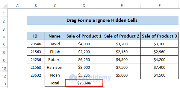
- Drag the Fill Handle icon to the right. It will drag formula horizontally with vertical reference and return the sum of product 2 and product 3. In all the cases, the function ignores the hidden cells.
- Copy the range of cell B4 to F13.
- Select cell B15 and paste it. It will display all the hidden cells with the updated sum value.
- To drag the formula ignoring hidden cells.
- Select the range of cells B4 to F13.
- Next, press ‘Alt+;’.
- Press Ctrl+C to copy the selected range of cells. It will highlight the cells.
- Select cell B15.
- Press Ctrl+V to paste the selected range of cells.
- The cells and formula ignores the hidden cells.
Read More: How to Enable Drag Formula in Excel
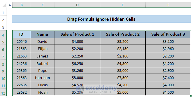
How to Drag Formula in Excel When Filtered
Steps
- Select the range of cells B4 to F12.
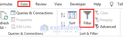
- Go to the Data tab in the ribbon.
- From Sort & Filter group, select Filter.
- It will filter your dataset.
- Select cell D13.
- Enter the following formula in the formula box
=SUBTOTAL(9,D5:D12)9 is the function_num which denotes the SUM function but will ignore unchecked filtered cells.
- Press Enter to apply the formula.
- Drag the Fill handle icon to the right. It will calculate the sum of product 2 and product 3.
- Click on the down arrow beside the Name
- Number Filter dialog box will appear.
- Uncheck Elijah, Noah, and Pope.
- Click on OK.
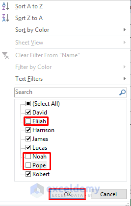
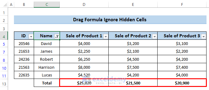
- It will filter the dataset and hide all the three names.
- It will change the overall sum of the three products because it allows only visible rows.
Download Practice Workbook
Related Articles
- How to Use Fill Handle in Excel
- How to Drag Cells in Excel Using Keyboard
- [Solved]: Fill Handle Not Working in Excel
- How to Use Fill Handle to Copy Formula in Excel
- How to Fill Formula Down to Specific Row in Excel
<< Go Back to Fill Handle in Excel | Learn Excel
Get FREE Advanced Excel Exercises with Solutions!
