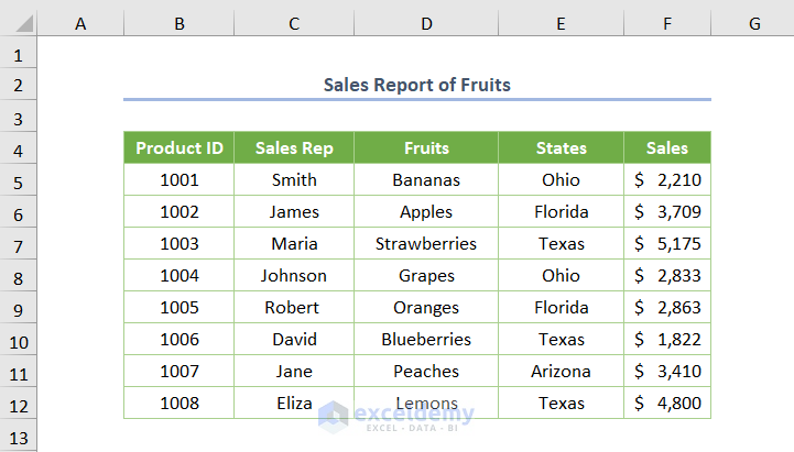
We have a dataset, Sales Report of Fruit, which shows Product ID, Sales Rep, Fruits, States, and Sales. We will show you how to drag the formula horizontally with vertical reference.
Method 1 – Using the COLUMN Function with VLOOKUP
Steps:
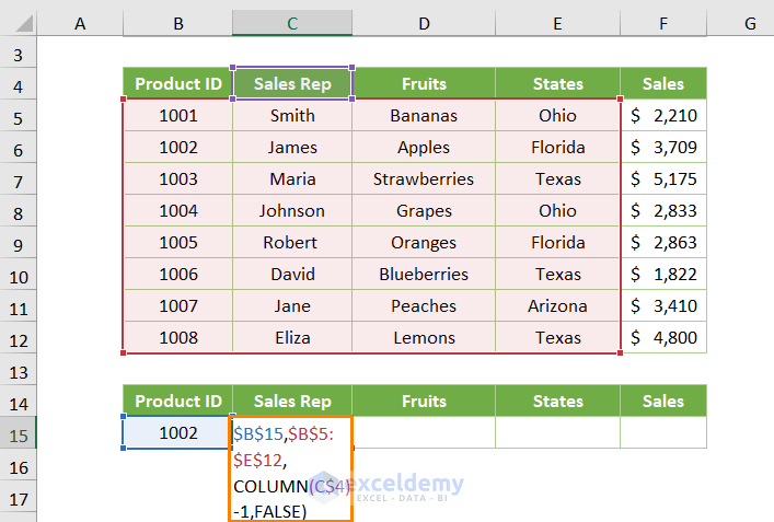
- Enter the following formula in cell C15:
=VLOOKUP($B$15,$B$5:$E$12,COLUMN(C$4)-1,FALSE)
Here, $B$15 is the lookup value, $B$5:$E$12 is the table_array argument, C$4 refers to the Sales Rep heading of column C, and FALSE is for the exact matching.
⧬ Formula Explanation:
- In the above formula, the COLUMN(C$4) syntax returns column number as 3 but you need to subtract 1 as the Sales Rep column is located at the 2nd position with respect to the lookup column (Product ID).
- Later, the VLOOKUP portion finds the relevant Sales Rep.
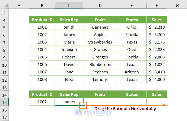
- Press ENTER and you’ll get the output as James.
- Drag the formula horizontally to pull out the other data for the specified Product ID.
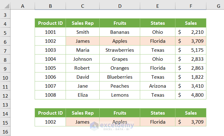
- The output will look as follows.
Read More: Excel Fill Down to Next Value
Method 2 – Using the INDEX Function
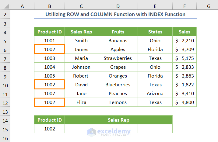
In the updated dataset, we used 1002 Product ID multiple times to extract the corresponding Sales Rep from different rows.
 Steps:
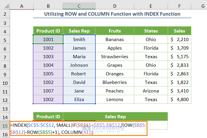
- Enter the following formula:
=INDEX($C$5:$C$12, SMALL(IF($B$15=$B$5:$B$12,ROW($B$5:$B$12)-ROW($B$5)+1), COLUMN(A1)))
Here, $B$5 refers to the starting cell of Product ID, $C$5:$C$12 is the cell range representing Sales Rep, and $B$5:$B$12 cells denotes Product ID.
⧬ Formula Explanation:
- The ROW function mainly finds the row number from a given range of datasets. Here, ROW($B$5:$B$12)-ROW($B$5)+1 returns the row number of the $B$5:$B$12 cells used as the 2nd argument of the IF logical function.
- Then, the IF($B$15=$B$5:$B$12, ROW($B$5:$B$12)-ROW($B$5)+1) executes searching to find the 1002 Product ID. When the formula matches, it returns TRUE, else it returns FALSE.
- The SMALL function finds the smallest value in a given dataset. Here, the function returns the lowest row number assigned as the row_num argument in the INDEX function.
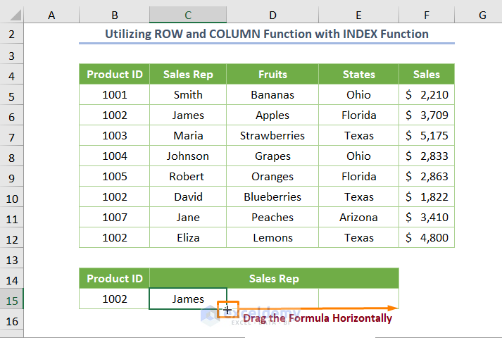
- Lastly, the INDEX function extracts the first Sales Rep for 1002 Product ID.
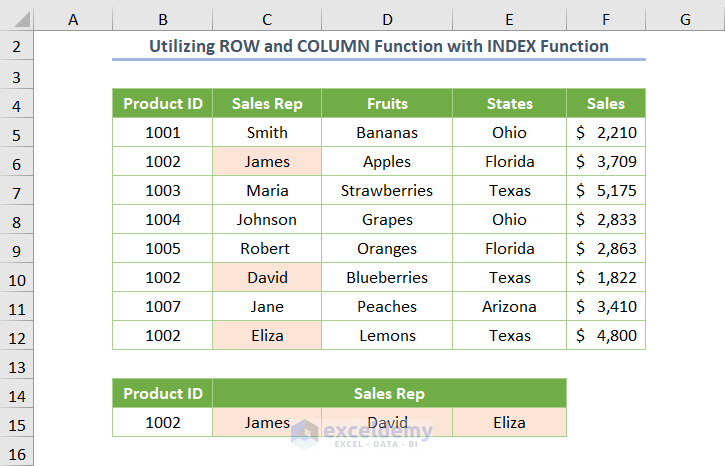
- Drag the formula horizontally to get the rest of the Sales Rep of the 1002 Product ID.
You’ll get the following output.
Read More: How to Drag Formula and Ignore Hidden Cells in Excel
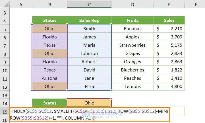
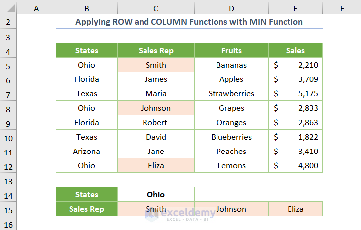
Method 3 – Applying ROW and COLUMN Functions with MIN Function
Steps:
- Enter the following formula:
=INDEX($C$5:$C$12, SMALL(IF($C$14=$B$5:$B$12, ROW($B$5:$B$12)-MIN(ROW($B$5:$B$12))+1, ""), COLUMN(A1)))
Here, the MIN function returns the lowest row number from the given $B$5:$B$12 cells. The rest work similarly, as discussed in the earlier method.
- Drag the formula horizontally.
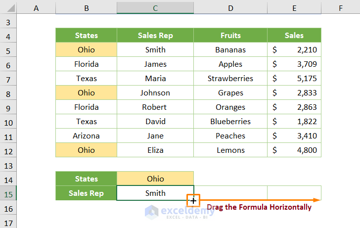
You’ll get the following output.
Read More: How to Fill Formula Down to Specific Row in Excel
Download the Practice Workbook
Related Articles
- How to Use Fill Handle in Excel
- How to Drag Cells in Excel Using Keyboard
- How to Drag Formula in Excel with Keyboard
- How to Enable Drag Formula in Excel
- [Solved]: Fill Handle Not Working in Excel
- How to Use Fill Handle to Copy Formula in Excel
<< Go Back to Fill Handle in Excel | Learn Excel
Get FREE Advanced Excel Exercises with Solutions!
