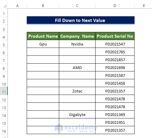
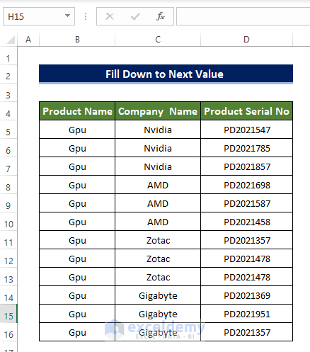
We have a sample dataset with products, companies that make variations of that product, and the serial models they make. There are blank cells in between the cells, which we’ll fill by filling existing entries down to the next values.
Method 1 – Using the Fill Handle
Steps
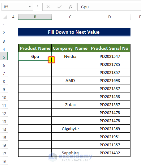
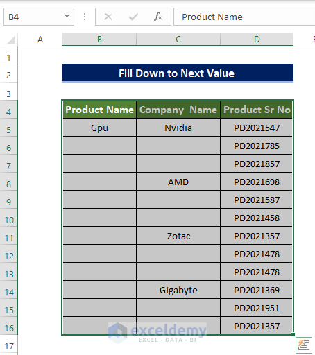
- Select the Fill Handle icon in the corner of cell B5 and drag it down to cell B17.
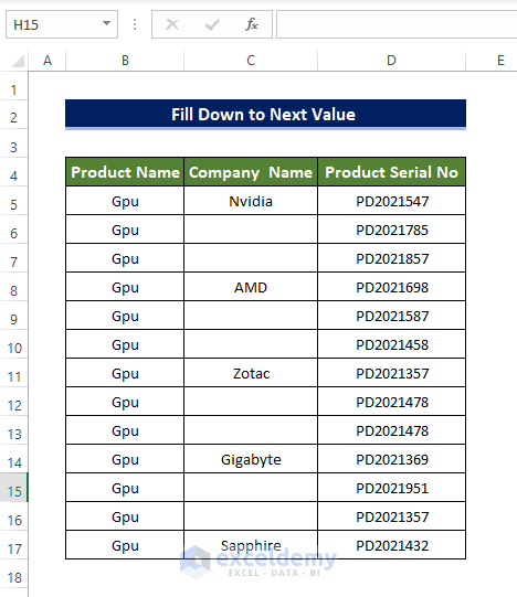
- The range of cells B4:B17 is now filled with the value of cell B5.
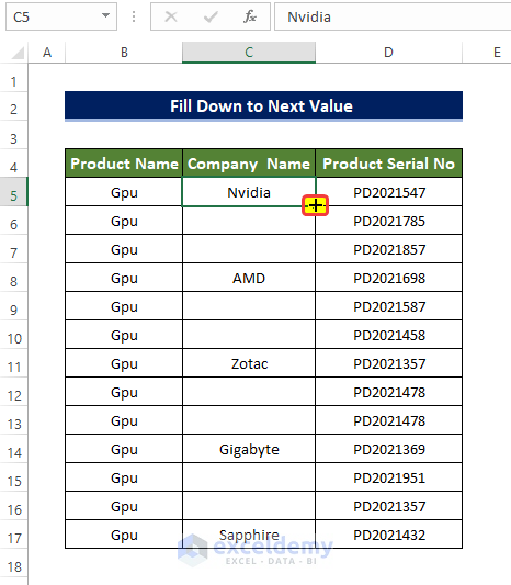
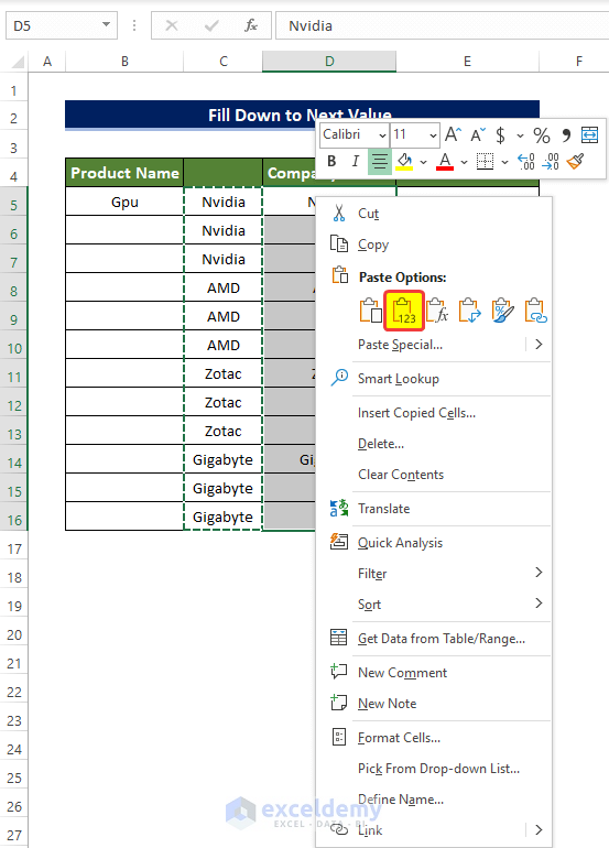
- Select cell C5 and drag the Flash Fill icon by pressing and holding the right mouse button instead of the left mouse button.
- Drag the Fill Handle to cell C7.
- Release the button. You will get a new context menu.
- Click on the Copy Cells.
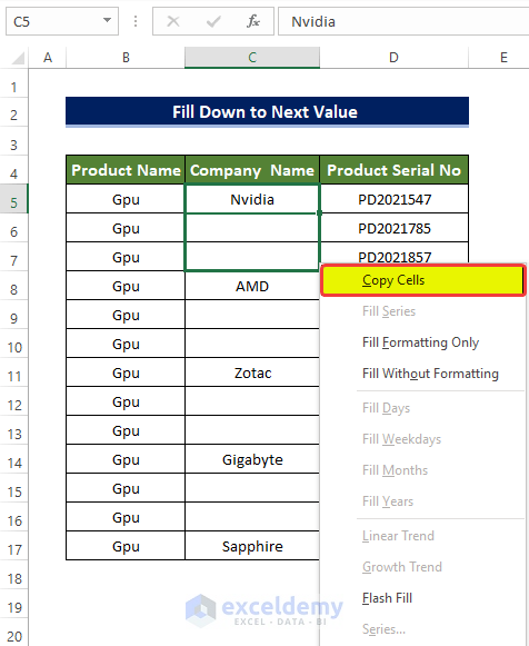
- You will notice that the range of cells C5:C7 now has Filled down with the value from cell C5.
- You can choose Flash Fill instead of Copy Cells to fill down the values as shown in the image below.
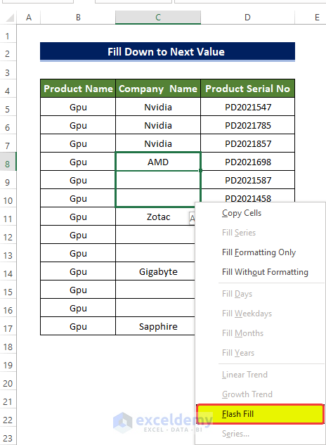
- Repeat for all values that you need to fill.
Note:
The Fill Handle button could be hidden in the worksheet. You can enable it via Advanced options in the Options menu in the File menu. In the Advanced options, go to Editing Options and check the Enable Fill Handle and drag-and-drop box.
Read More: How to Enable Drag Formula in Excel
Method 2 – Utilizing the Go To Special Command
Steps
- Select the range of cells B4:D16 and press on F5.
- You will get a new window named Go To.
- Click on Special.

- You will get another window named Go To Special.
- Select Blanks and click on OK.
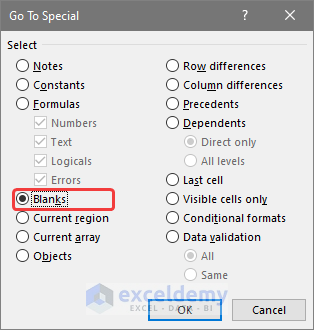
- All of the blank cells in the range of cells B4:D17 are now selected.
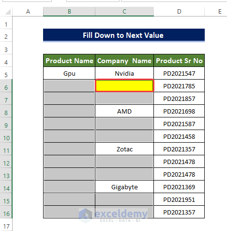
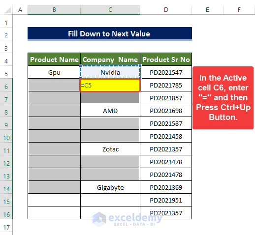
- Enter “=” in the active cell C6, then press the Up arrow on the keyboard.
- This will select cell C5.
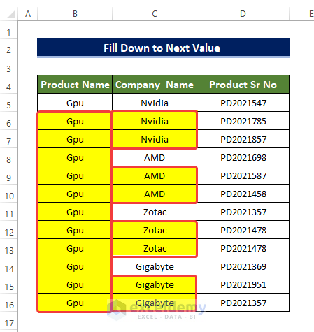
- Press Ctrl + Enter on the keyboard.
- The blank cells are now filled down with the next value of their upper cells.
Read More: How to Drag Cells in Excel Using Keyboard
Method 3 – Applying Power Query
Steps
- Click on From Table/Range from the Data tab.
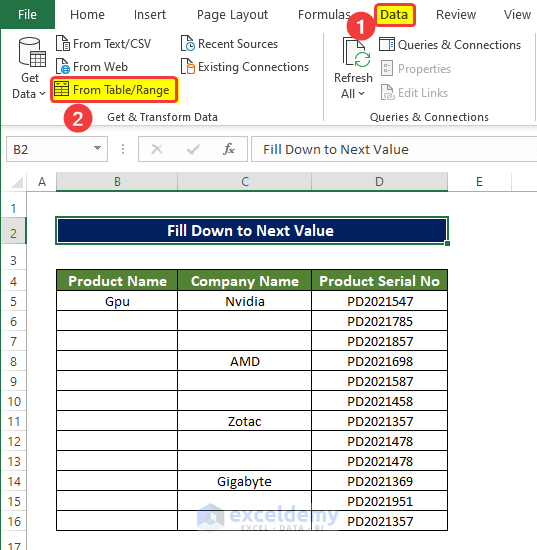
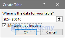
- You will get a small window asking for the range of your table, which you want to add.
- Input $B$4:$D$16, and tick on the My table has headers box. Alternatively, you can select the data range before choosing the From Table/Range option.
- Click OK.
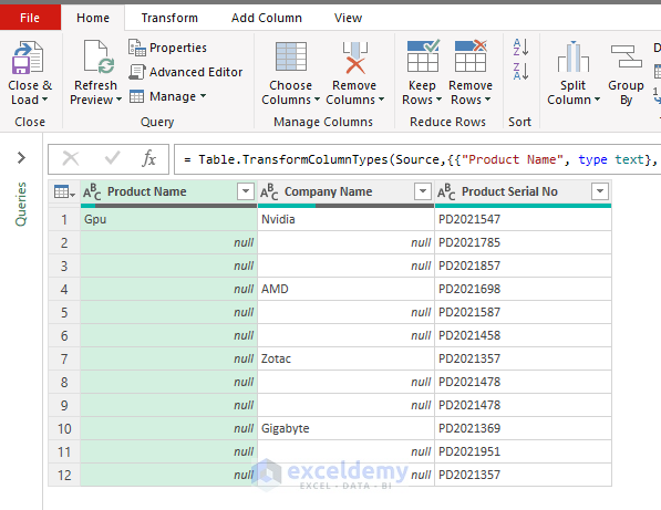
- You’ll get a new Power Query window with loaded values. The empty cells are showing null.
- Right-click on the company name column, go to Fill, and select Down.
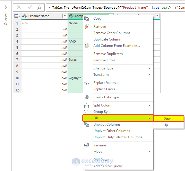
- The company name column is now filled down with the next cell values from the upper cells.
- Right-click on the Products Name column, go to Fill, and select Down.
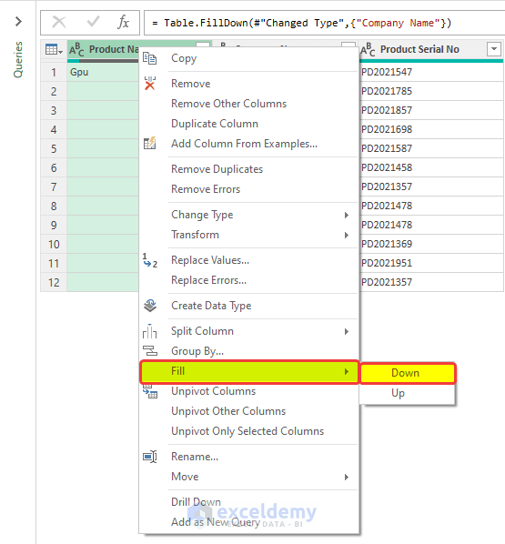
- The whole table is now filled down with the next value in the upper cells.
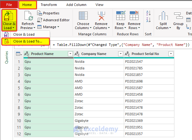
- Click on the Close & Load icon from the Home tab and then click on Close and Load To.
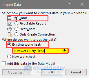
- You will get an Import Data dialog box.
- Click on Table.
- Select Existing Worksheet in the Where do you want to put the data? option.
- Select the location in the range box. We entered F4 in the box.
- Click OK.
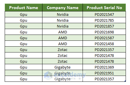
- The range of cells F4:H16 is now occupied with the table that we just modified in Power Query.
Read More: How to Drag Formula and Ignore Hidden Cells in Excel
Method 4 – Using the IF Function
Steps
- The range of cells D5:D16 has been copied to the range of cells C5:C16.
- Select cell C6 and enter the following formula.
=IF(D6="",C5,D6)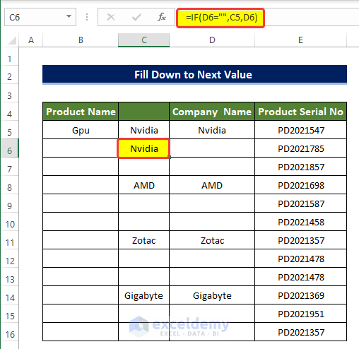
- Drag the fill handle down to cell C16.
- The range of cells C5:C16 is filled down with the next upper cell value.
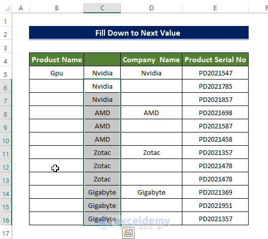
- Cut the range of cells C5:C16 and copy them onto D5:D16.
- Copy the cell B5 into C5.
- Select cell B6 and enter the following formula:
=IF(C6="",B5,C6)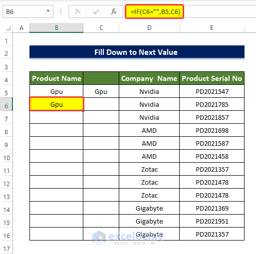
- Drag the Fill Handle down to B16.
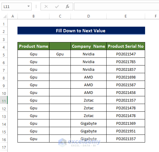
- The range of cells B5:B16 is now filled down to the next upper value.
Read More: How to Drag Formula Horizontally with Vertical Reference in Excel
Method 5 – Embedding VBA Macro
Steps
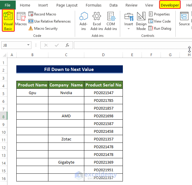
- From the Developer tab, go toVisual Basic.
- Click Insert and choose Module.
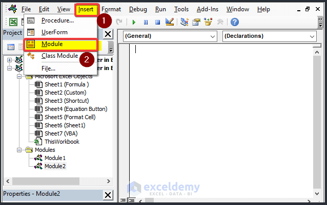
- In the module window, enter the following code.
Sub Down_Fill_next_value()
Dim x As Range
Dim y As Long, z As Long
Dim m As Integer, n As Integer
Set x = Selection
z = x.Columns.CountLarge
y = x.Rows.CountLarge
For n = 1 To z
  For m = 1 To y - 1
    If x.Cells(m, n) <> "" Then
      x.Cells(m, n) = x.Cells(m, n).Value
      If x.Cells(m + 1, n) = "" Then
        x.Cells(m + 1, n) = x.Cells(m, n).Value
      End If
    End If
  Next m
Next n
End Sub
- Close the window.
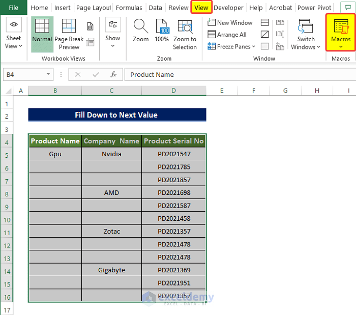
- Select the range of data that you need to fill with the next cell value.
- Go to the View tab and select Macros.
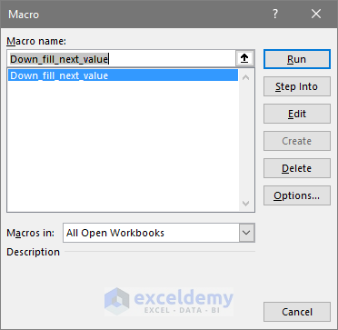
- Select the macro that you created named Down_Fill_next_value.
- Click Run.
- Here are the results.
Read More: How to Use Fill Handle in Excel
Download the Practice Workbook
Download this practice workbook below.
Related Articles
- How to Drag Formula in Excel with Keyboard
- How to Fill Formula Down to Specific Row in Excel
- [Solved]: Fill Handle Not Working in Excel
<< Go Back to Fill Handle in Excel | Learn Excel
Get FREE Advanced Excel Exercises with Solutions!
