Method 1 – Applying INT and MOD Functions
Steps:
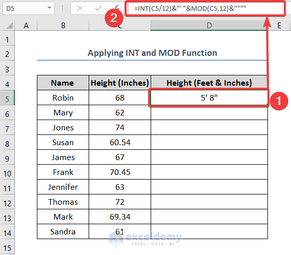
- Select cell D5, type down the formula below, and press ENTER to get the result in feet and inches.
=INT(C5/12)&"' "&MOD(C5,12)&""""
Formula Breakdown:
The formula converts the numeric value of inches to text representing the same amount in inches and feet.
Use the INT function to get the value for feet. The formula for this part is as below:
=INT(C5/12)&"' "
In the INT function, inside the parentheses, the value in cell C5 is divided by 12 as 1 foot is equal to 12 inches. INT function simply rounds down to its nearest integer value. It returns the integer part of the number, removing any decimal portion.
A single quote is put inside a quotation mark to mean feet sign, with an ampersand (&) operator concatenated with the INT function.
The next part of the formula is as below:
=MOD(C5,12)&""""
The MOD function returns the remainder after division. The value in cell C5 is the dividend, and 12 is the divisor.
This result is concatenated with two pairs of double quotes. The outer pair is for indicating text and the inner pair is to indicate the inch symbol.
Both the functions are concatenated with the ampersand operator
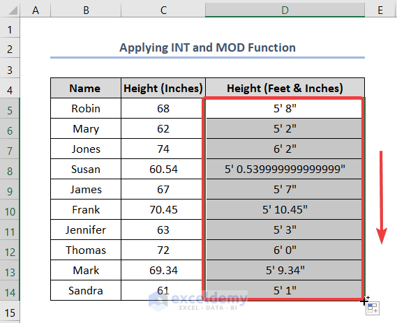
- Get the cursor at the bottom right part of cell D5 and use the Fill Handle tool to copy the formula in other cells with a view to getting the values of these cells in feet and inches.
Method 2 – Converting Inches to Feet and Inches with Labels
- Select cell D5, write down the formula below, and press ENTER.
=INT(C5/12)&"ft. "&MOD(C5,12)&"in."
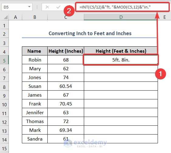
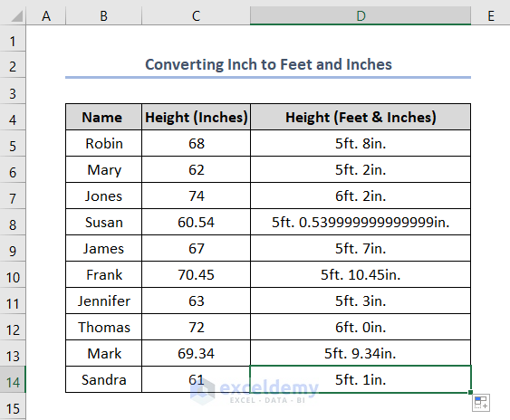
Notice that with our previous formula, the only difference is that we interchanged the “single quote” and “double quote” with “ft.” and “in.”. It displays ft. and in. instead of a quote sign.
Method 3 – Utilizing the ROUND Function to Convert Inches
Steps:
- Cell D5, put down the formula below, and ENTER. Use the Fill Handle tool and drag it down to get the whole results.
=INT(C5/12)&"' "&ROUND(MOD(C5,12),2)&""""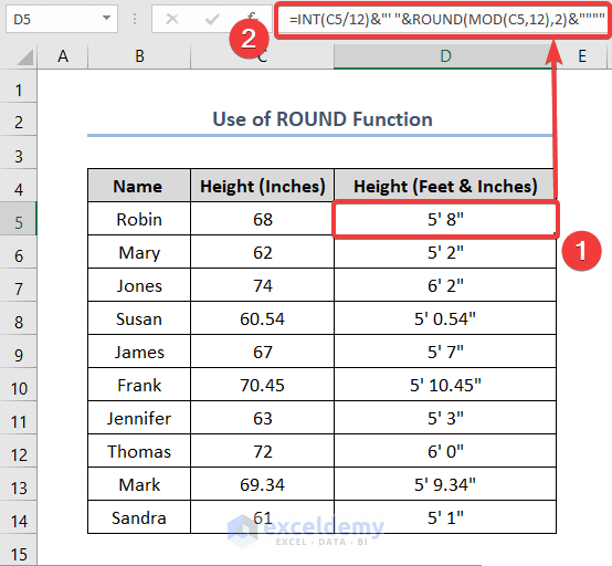
The MOD function returns the remainder after division and the ROUND function returns the decimal value to 2 digits. These heights in feet and inches look pretty much presentable.
Method 4 – Converting Inches to Feet and Inches If the Input Is Negative
- Choose cell D5 and type down the formula as follows, press ENTER.
=TRUNC(C5/12)&"' "&ROUND(MOD(ABS(C5),12),2)&""""
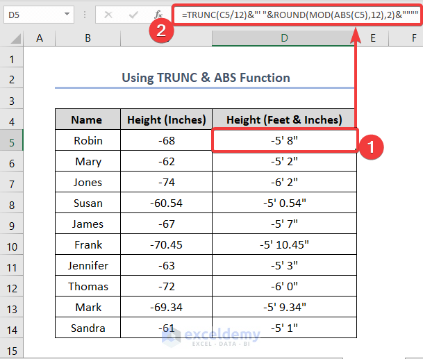
Use the ABS function to ensure that the integer inside MOD is positive and as well as replace INT with the TRUNC function. The INT function rounds negative numbers down away from zero. TRUNC function, on the other hand, removes the decimal value and leaves the integer along with the sign. The MOD function also doesn’t work correctly with negative numbers. Using the ABS function, we will get the absolute value always to work with the MOD function. This formula can completely run with both positive and negative numbers.
Method 5 – Using CONVERT Function to Transform Inches
Steps:
- Select cell D5, and write down the formula below and press ENTER.
=ROUND(CONVERT(C5,"in","ft"),3)
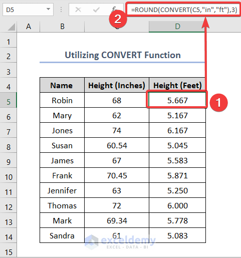
We took the value from cell C5 as a number and converted it from inches to feet. Using the ROUND function, round up the decimal value to 3 digits to look clean.
- Select cell E5 paste the formula below, and press ENTER.
=TRUNC(D5)&"' "&ROUND((D5-TRUNC(D5))*12,2)&""""
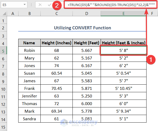
We used the TRUNC function. To get the inches part, we must multiply the decimal portion of cell D5 with 12. We subtracted the integer part from the whole number of cell D5 and multiplied it by 12. At last round down the decimal number to 2 digits to give it a cleaner look. The feet and inch signs are put as our previous methods.
Things to Remember
- In the result, we got our measurements in feet and inches in text format. So, we cannot use these cell references as values in other formulas.
Download Practice Workbook
You may download the following Excel workbook for better understanding and practice yourself.
Related Articles
- How to Convert inch to mm in Excel
- How to Convert Units in Excel
- How to Convert Inches to Meters in Excel
- How to Convert Feet and Inches to Decimal in Excel
- How to Convert Millimeters (mm) to Inches (in) in Excel
- How to Convert Millimeters (mm) to Feet (ft) and Inches (in) in Excel
<< Go Back to Excel CONVERT Function | Excel Functions | Learn Excel
Get FREE Advanced Excel Exercises with Solutions!

Nice writing. Actually my ques is out of this topic. But I’m facing this problem severely in my spreadsheet. In some cells of my sheet, there are some extra spaces, but i cannot figure out how to remove them automatically. This creates error in calculations also. Could you help on this?
Hello JACOB,
Thanks for your appreciation first. Now coming back to your question. I understood your problem easily. It takes a great effort if you try to remove those extra spaces manually from the cells one by one. But no problem. We have a smart workaround for you. Just follow the following steps.
We can see that there are some spaces in cells in the C5:C8 range which we want to remove.
• Firstly, press CTRL+F on your keyboard.
• Immediately, the Find and Replace dialog box appears
• Secondly, go to the Replace tab.
• In the Find what box, type down a single blank space.
• Keep the Replace with box blank.
• After that, click on the Replace All button.
Instantly, it’ll show a message box with the message “All done. We made 20 replacements.”. Also, the extra spaces are gone in the dataset.
Additionally, you can go through the article How to Remove Blank Spaces in Excel in our website to know more techniques regarding this problem. Also, follow our website, ExcelDemy, a one stop Excel solution provider to explore more. Happy Excelling.
Hello.
Thank you for sharing your skills.
I am looking for a formula to convert a decimal inch value to fractional feet & inches, i.e 19.125″ to 1′ 7 1/8″ The =INT(C5/12)&”‘ “&ROUND(MOD(C5,12),2)&”””” formula comes close, but the result is 1’7.13″
How do I modify the formula to display what I need?
I am an Excel novice.
Thank you.
Hello Stephen,
Thank you for your kind words. To convert a decimal inch value like 19.125 into 1′ 7 1/8″, you need to convert the decimal part of the inches into a fraction.
You can use this formula:
=INT(C5/12)&”‘ “&INT(MOD(C5,12))&” “&TEXT(MOD(C5,1),”# ?/?”)&””””
For 19.125, this returns: 1′ 7 1/8″
Here, INT(C5/12) returns the feet, INT(MOD(C5,12)) returns the whole inches, and TEXT(MOD(C5,1),”# ?/?”) converts the decimal inch part into a fraction.
Regards,
ExcelDemy
Hello, Shamima,
Thank you for the response.
I copied your formula into a cell, and Excel displayed a dialog stating that there were punctuation errors. I am unable to paste a copy of the error here.
I put the value I wish to change into cell C5, so that I did not have to modify the formula.
TIA
Hello Stephen,
Thank you for letting me know. The issue is likely due to the quotation marks being converted when copied from the website or comment section.
Please try typing the formula directly into Excel rather than copying it from the comment.
You can also try this version:
=INT(C5/12)&”‘ “&TEXT(MOD(C5,12),”# ?/?”)&””””
For a value of 19.125 in C5, the result should be: 1’ 7 1/8″
If you still receive an error, could you please let me know:
1. Your Excel version (Excel 365, 2021, 2019, etc.)
2. Whether your formulas use commas (,) or semicolons (;)
That will help me provide the exact formula for your setup.
Regards,
ExcelDemy
Thank you for this.
Excel returns a punctuation error.
Hello Stephen,
Thank you for checking again. Please try this simpler formula:
=TEXT(C5/12,”#’ ?/12″)
However, for the exact format 1′ 7 1/8″, this formula should work better:
=INT(C5/12)&”‘ “&TEXT(MOD(C5,12),”# ?/?”)&””””
If Excel still shows a punctuation error, please manually replace the last part &”””” by typing four double quotation marks from your keyboard. Sometimes copied quotation marks from web comments become “smart quotes,” and Excel cannot read them.
Regards,
ExcelDemy
Hello, Shamima.
Thank you for the suggestion, however, retyping those characters resulted in the same error. I thought that there may be other character issues, so I retyped the entire formula and was able to get it to work! Yes!!
One minor issue is that the results I am getting do not fit with my industry. I tested the formula on a value I needed to convert, 2777.689″, and the result came back as 231′ 5 2/3″. This is close, but I need to provide values rounded to a 1/16″ or 1/32″. Can this be done?
Thank you.
Also, I am not sure why this is happening but I find that I need to post my questions twice before they appear here.
Hello Stephen,
I’m glad you were able to get the formula working! Yes, the fraction can be rounded to a specific denominator such as 1/16″ or 1/32″. The formula I provided uses Excel’s default fractional formatting, which may return values such as 5 2/3″ rather than the construction-style fractions commonly used in industry.
For example, to round the inch portion to the nearest 1/16″, you can first round the value:
=ROUND(C5*16,0)/16
and then convert the result to feet and inches.
For your example of 2777.689″, rounding to the nearest 1/16″ would give a result closer to the format typically used in construction, woodworking, and manufacturing applications.
As for having to post twice, that is likely related to the website’s moderation or approval process rather than anything in Excel.
Thank you for testing the formulas and providing feedback. I’ll see if I can come up with a cleaner single-cell formula that always returns feet and inches rounded to a specified fraction such as 1/16″ or 1/32″.
Regards,
ExcelDemy