Excel is the most widely used tool for dealing with massive datasets. We can perform myriads of tasks of multiple dimensions in Excel. Sometimes, we need to determine dates that are older than 1 year for our calculation. We can easily do it in Excel. In this article, I will show you the methods in Excel for conditional formatting based on dates older than 1 year in Excel. There are 3 methods in this article.
Conditional Formatting Based on Date Older Than 1 Year in Excel: 3 Easy Methods
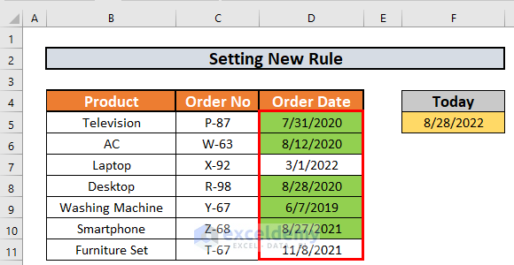
This is the dataset for today’s article. We have some products along with their Order Number and Order Date. I will find out the dates that are older than 1 year using conditional formatting.
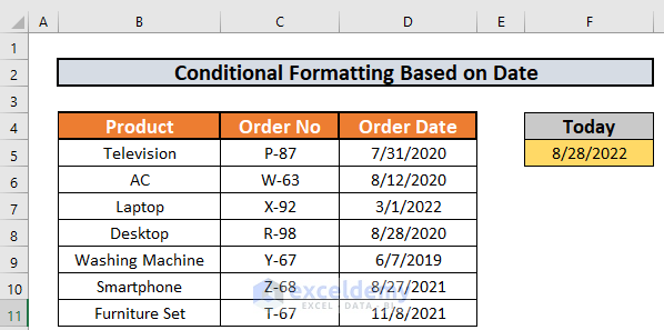
I have mentioned today’s date just for convenience. This will not have any effect on the process.
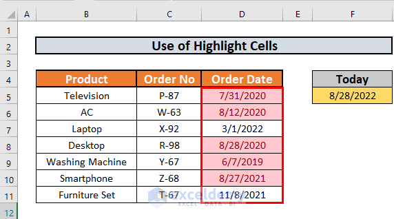
1. Use of Highlight Cells Option
First of all, I will show how to use the Highlight Cells Option to find out the dates older than 1 year. In this method, I will use the TODAY function.
Steps:
- First, select the range D5:D11.
- Then, go to the Home
- After that, go to Conditional Formatting.
- Then, select Highlight Cells Rules.
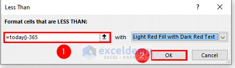
- Finally, choose Less Than…

- A box will appear. Write down the following formula in the box
=today()-365- Then, press OK.
- Excel will find out the dates older than today.
2. Set New Rule Based on Date Older Than 1 Year
You can also find out the dates older than 1 year by setting a new rule in conditional formatting. Let me show you how to do so step by step.
Steps:
- First of all, select the range D5:D11.
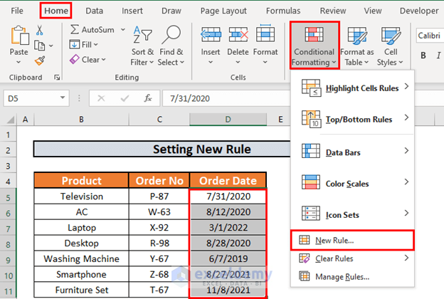
- Then, go to the Home
- After that, select Conditional Formatting.
- Finally, select New Rule.
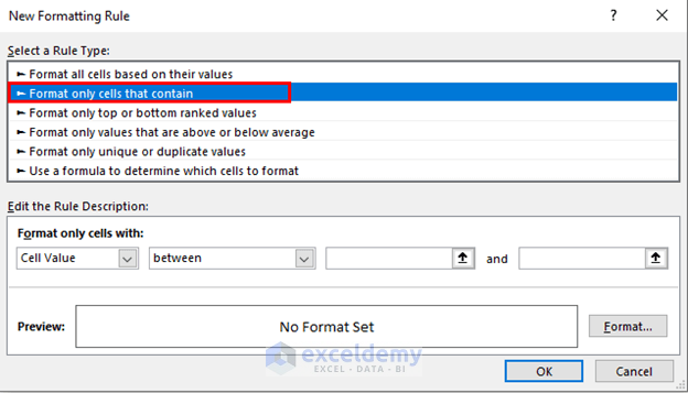
- A box will appear. Select Format only cells that contain.
- Then, choose less than from the drop-down list.
- After that, write down the following formula
=today()-365 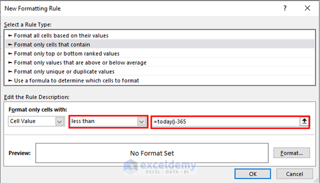
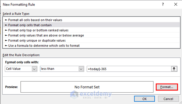
- Then, you need to format the cells that have dates older than 1 year. For this, select Format.
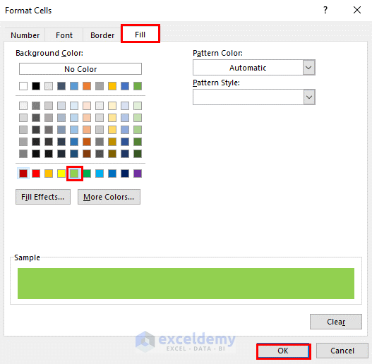
- Format the way you want. I will change the Fill color.
- Click OK.
- Then, click OK.

- Excel will format dates older than 1 year.
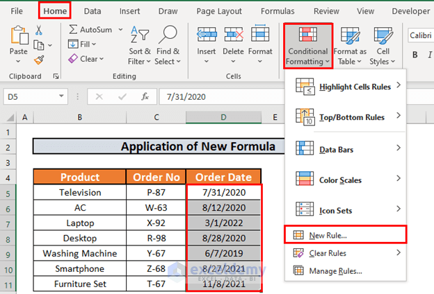
3. Apply New Formula to Apply Conditional Formatting
The next method is applying a new formula in conditional formatting. Let’s do it step by step.
Steps:
- First of all, select the range D5:D11.
- Then, go to the Home
- After that, select Conditional Formatting.
- Finally, select New Rule.
- A box will appear. Select Use a formula to determine which cells to format.
- Then, write down the formula
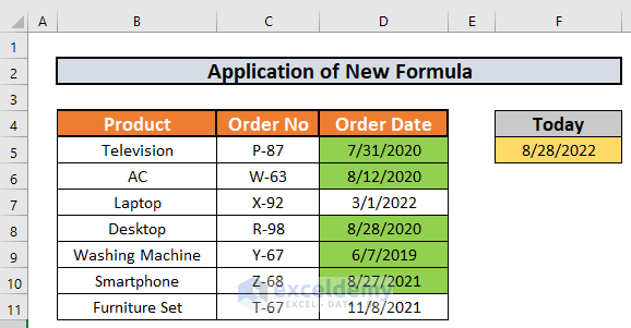
=D5<=TODAY()-365- Then, click OK.

- Excel will do the formatting. The output will be like this.
Things to Remember
- The day when you use the TODAY function will be considered today in Excel.
Download Practice Workbook
Download this workbook and practice while going through the article.
Conclusion
In this article, I have shown 3 methods in Excel for conditional formatting based on dates older than 1 year in Excel. I hope it helps everyone. If you have any suggestions, ideas, or feedback, please feel free to comment below.
<< Go Back to Dates | Compare | Learn Excel
Get FREE Advanced Excel Exercises with Solutions!
