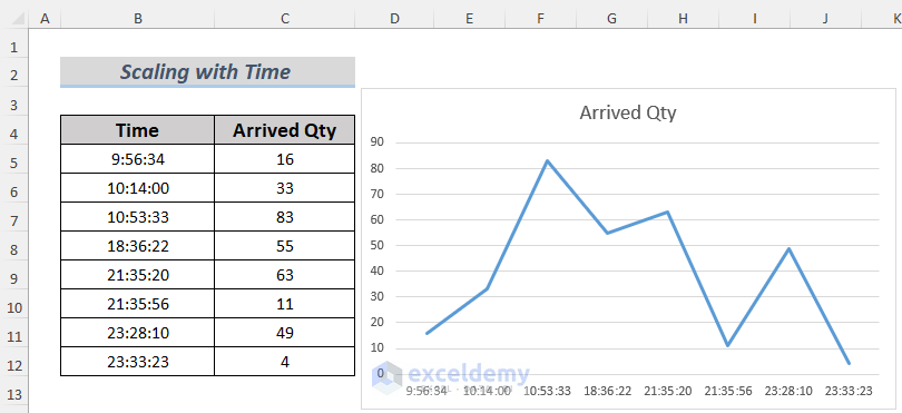
Generally, if you use a Line Chart, it works fine. Let’s have a look at the following picture.
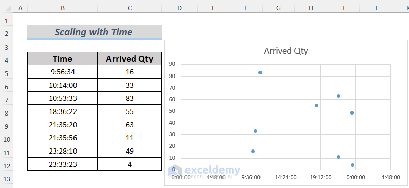
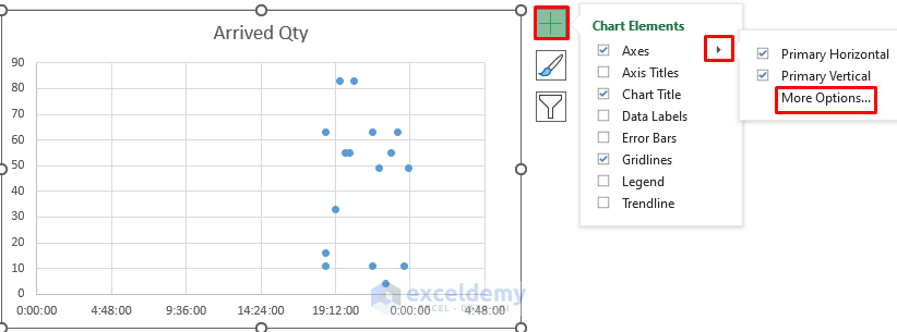
If we create a Scatter Chart based on this dataset, you may find the chart inconvenient. The axis starts from the zero hour (12:00 AM or 0:00) and there are some unnecessary gaps in the chart.
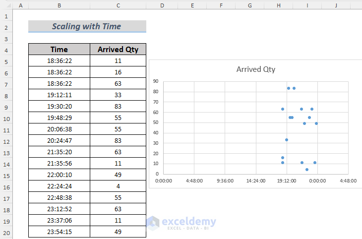
This becomes more inconvenient if the dataset contains more time values.
We will show you how to get rid of this problem.
Method 1 – Scaling the Time in the X-Axis in an Excel Chart
Steps:
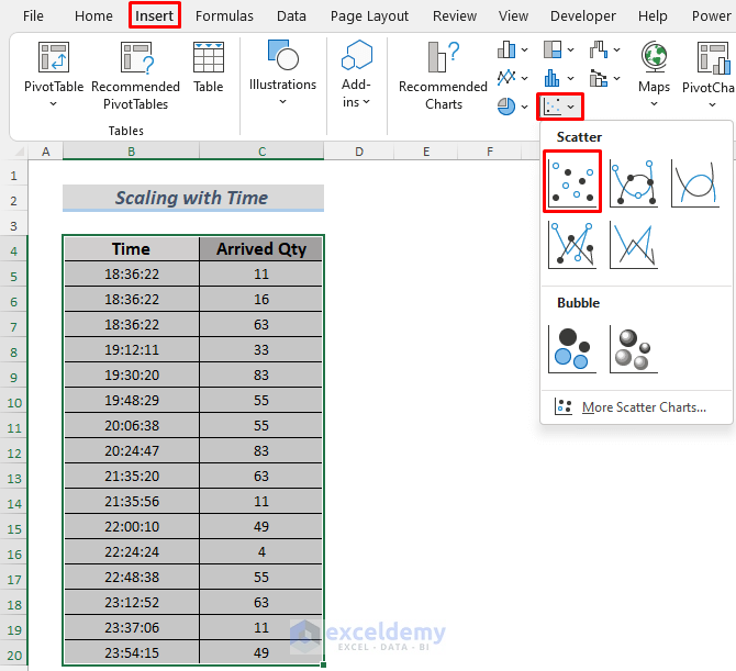
- Select the data range (B4:C20) and then go to Insert, then Chart, and select Scatter Chart.
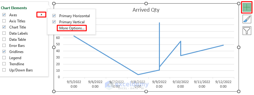
- Click on the plus icon of the chart, go to Axes and choose More Options.
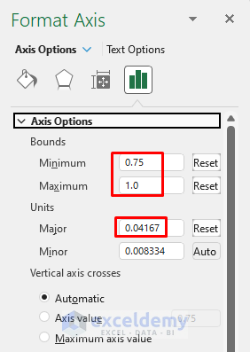
- The Format Axis window will appear. Insert the values like the following image.
In the Bounds section, the Maximum value represents 24 hours which is 1 unit. So, 1 hour becomes 1/24 = 0.04167 units. As the time data here starts at around 18:30, the minimum value becomes 18.5*0.04176 = 0.75.
That’s why we set the Minimum Bound value to 0.75 and the Maximum Bound value to 1.0. As 1 hour equals 0.04167 units, we set Major Unit to this value. The Minor Unit value becomes 0.008334 automatically by default.
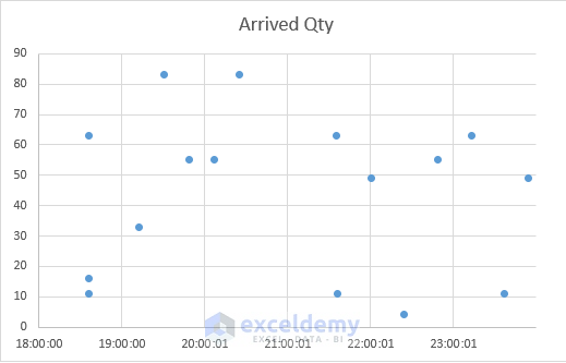
The Scatter Chart looks more convenient and easily understandable.
Method 2 – Scaling the Time in X-Axis by the Date in an Excel Chart
Steps:
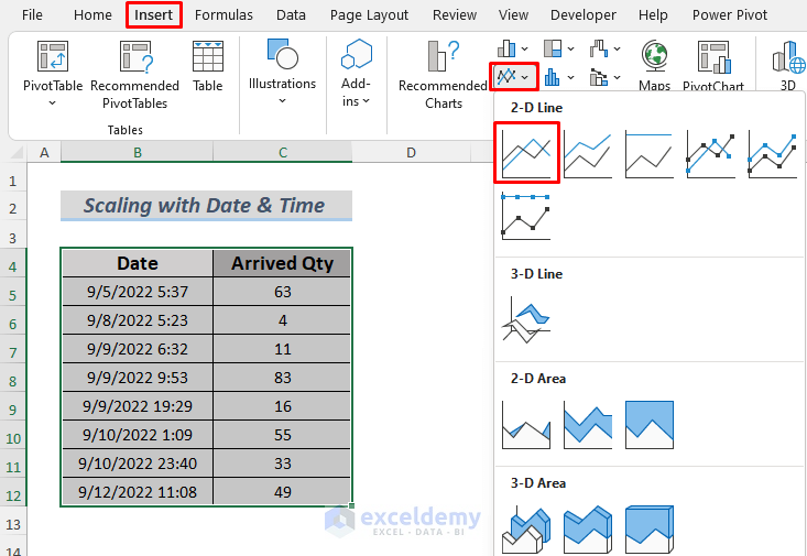
- Select the data and go to Insert, then to Chart, and choose Line Chart.
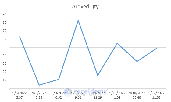
- You will see that there is a vertical line on the date 9th September although this date has two different data points. Click on the plus icon of the chart and select Axes, then More Options.
- Change the Axis Type to the Text axis.
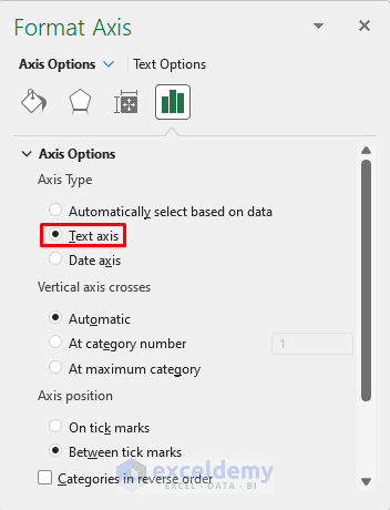
- You will see that the chart shows different data for 9th September.
Method 3 – Changing the Number Format
Steps:
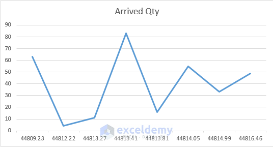
- Create a Line Chart following the process of Method 2.
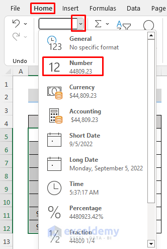
- Change the format of the Date column to Number from the Number group of the Home Tab. You need to select the range B5:B12 and then click on the drop down icon of the Number group and select the General or Number option.
- You will see separate data for 9th September. But, you may find it inconvenient, as the date on the horizontal axis is turned into numbers.
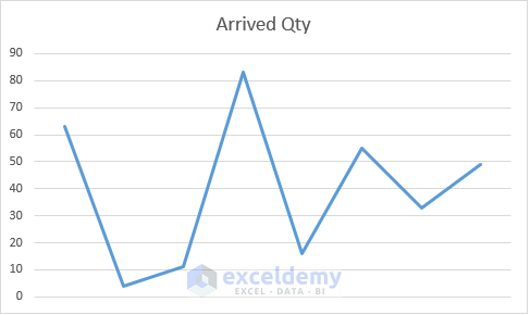
- Click on the plus icon of the chart and select Axes, then uncheck Primary Horizontal.
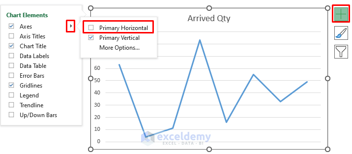
- This will remove the horizontal labels and gives you a better view of the chart.
Download the Practice Workbook
Related Articles
- How to Change Axis Scale in Excel
- Automatic Ways to Scale Excel Chart Axis
- How to Set Logarithmic Scale at Horizontal Axis of an Excel Graph
- How to Change Axis to Log Scale in Excel
- How to Break Axis Scale in Excel
- How to Set Intervals on Excel Charts
<< Go Back to Excel Axis Scale | Excel Charts | Learn Excel
Get FREE Advanced Excel Exercises with Solutions!
