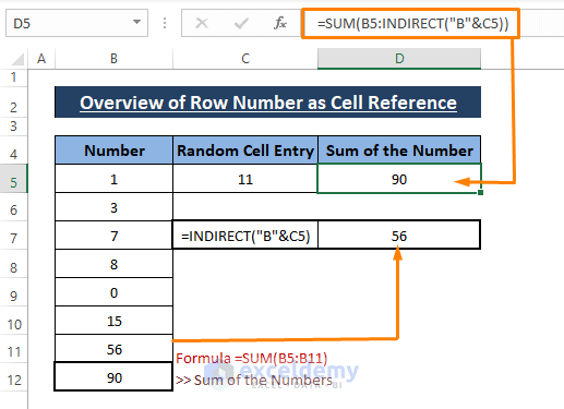
As shown in the below screenshot, we want the sum of a couple of numbers. We can simply get the sum by summing the range (i.e., B5:B11). However, if we can’t insert B11 as cell reference then we use a random row number (i.e.C5). The INDIRECT, OFFSET, or INDEX function converts the C5 cell value 11 as B11 cell reference. The overall conversion becomes B(C5)=B11.
How to Use Variable Row Number as Cell Reference in Excel: 4 Easy Ways
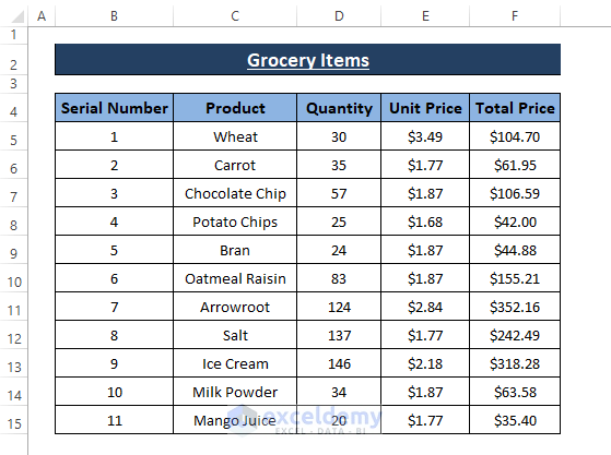
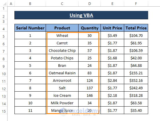
Our dataset contains Serial Number as row number and other columns as shown in the following picture. We want the sum of Total Price using variable row number as a cell reference.
Method 1 – The INDIRECT Function to Enable a Variable Row Number as a Cell Reference
The INDIRECT function returns a cell reference taking the text as arguments. The syntax of the INDIRECT function is
=INDIRECT (ref_text, [a1])ref_text; reference in a text string
[a1]; boolean indication of cell A1. TRUE (by default) = cell A1 style. [optional]
Steps:
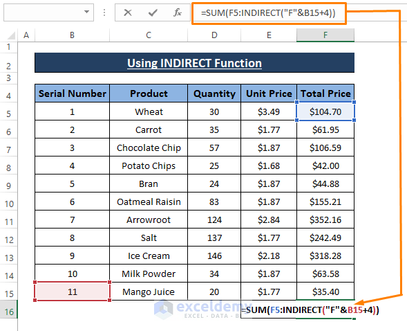
- Paste the following formula in the respective cell (i.e., F16).
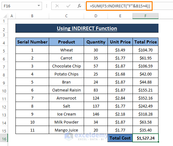
=SUM(F5:INDIRECT("F"&B15+4))The SUM function formula simply sums the range (i.e., F5:F15). But first, the INDIRECT function takes the B15 cell value (i.e.,11) then adds 4 to make it 15. At last, INDIRECT passes it as F15 to the formula. As a result, F(B15) becomes F(11+4)=F15
- Press Enter.
Read More: How to Display Text from Another Cell in Excel
Method 2 – Insert a Variable Row Number as a Cell Reference Using OFFSET
Similar to the INDIRECT function, the Excel OFFSET function also returns cell reference. The syntax of the OFFSET function is
=OFFSET (reference, rows, cols, [height], [width])reference; starting cell from where the row and column number will be counted
rows; number of rows below the reference.
cols; number of columns right to the reference.
height; number of the rows in the returned reference. [optional]
width; number of columns in the returned reference. [optional]
Steps:
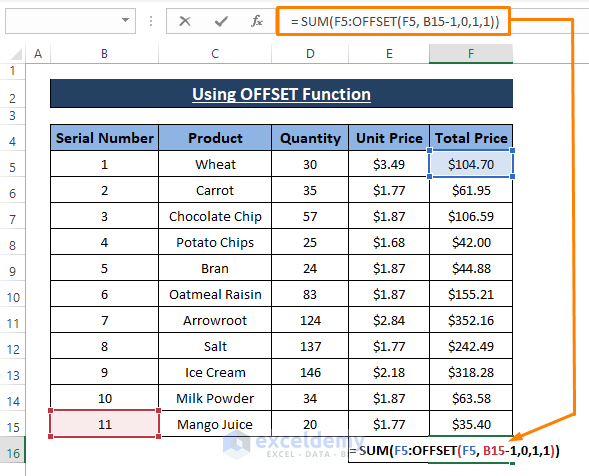
- Use the below formula in the cell F16.
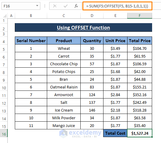
= SUM(F5:OFFSET(F5, B15-1,0,1,1))In the above formula, the OFFSET function takes F5 as a cell reference, B15-1 (i.e., 11-1=10) as variable rows, 0 as cols, 1 as height and width. By changing the B15 or B15-1 you can insert any number as the cell reference.
- Hit Enter to display the total sum.
Read More: How to Reference Text in Another Cell in Excel
Method 3 – INDEX Function to Use a Variable Row Number
The INDEX function results in values of the assigned location. The syntax of the INDEX function is
=INDEX (array, row_num, [col_num], [area_num])array; range or array.
row_num; row number in the range or array.
col_num; column number in the range or array. [optional]
area_num; range used in the reference. [optional]
Steps:
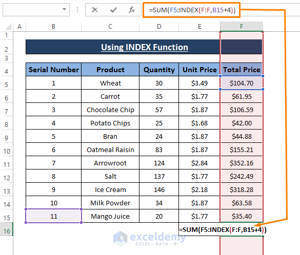
- Use the following formula in any blank cell (i.e., F16)
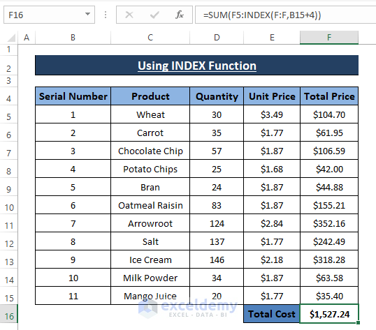
=SUM(F5:INDEX(F:F,B15+4))The INDEX function considers the F (i.e., F:F) column as an array, B15+4= 15 as the row_num. Other arguments are optional so it’s not necessary to use them. The INDEX(F:F,B15+4) portion in the formula returns $35.4 (i.e., F15 cell value). Changing B15 or B15+4 results in variable row numbers in the formula.
- Use the Enter key to get the result.
Read More: How to Reference Cell by Row and Column Number in Excel
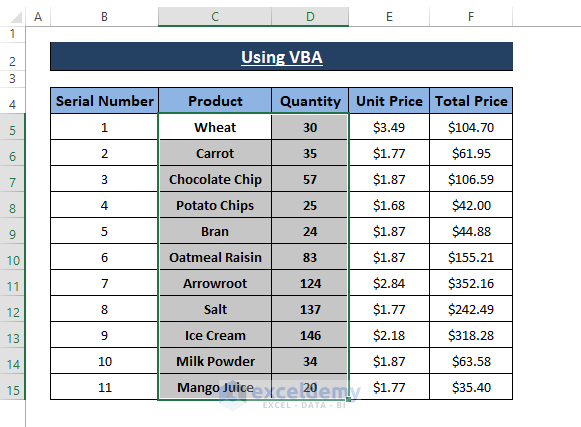
Method 4 – VBA Macro to Take a Variable Row Number as a Cell Reference
Suppose we want to highlight specific rows (i.e., C5:D15) as shown in the following image in bold.
Steps:
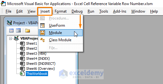
- Press Alt + F11 to open the Microsoft Visual Basic window.
- Select Insert (from the Toolbar) and click on Module.
- Paste the following macro in the Module.
Sub Row_variable()
Dim R_num As Integer
R_num = InputBox("Provide Preferred Row Number")
Sheets("VBA").Range(Cells(R_num, 3), Cells((R_num + 10), 4)).Select
Selection.Font.Bold = True
End Sub 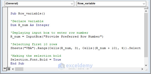
The macro code takes a row number using a VBA Input Box then highlights the first 10 rows. The highlight is done using VBA Selection.Font.Bold property.Sheets.Range statement assigns a specific sheet and range. Also, it defines the range using the VBA CELL property.
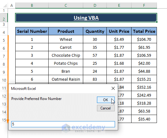
- Use the F5 key to run the macro.
- The macro displays an input box and asks to enter a row number.
- Enter the row number (i.e., 5) and click on OK.
- Clicking OK takes you to the Module window.
- Return to the worksheet.
- You see the assigned range (i.e., C5:D15) gets highlighted in Bold.
Read More: How to Find and Replace Cell Reference in Excel Formula
Download the Excel Workbook
Related Articles
- How to Use Cell Value as Worksheet Name in Formula Reference in Excel
- How to Use OFFSET for Cell Reference in Excel
- How to Reference a Cell from a Different Worksheet in Excel
- How to Reference Cell in Another Sheet Dynamically in Excel
- Excel VBA Examples with Cell Reference by Row and Column Number
- Excel VBA: Cell Reference in Another Sheet
<< Go Back to Cell Reference in Excel | Excel Formulas | Learn Excel
Get FREE Advanced Excel Exercises with Solutions!
