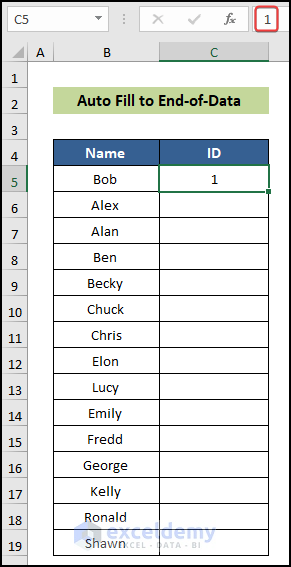
Method 1 – Autofill to End-of-Data
We have a set of names in the Name column. We need to assign an ID serially.
Steps:
- Select cell C5.
- Write down the first ID in that cell. We wrote 1.
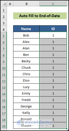
- Double-click the Fill Handle icon to fill in all the relevant cells in a column.
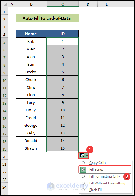
- Click on the Auto Fill Options icon on the bottom-right and choose the Fill Series option.
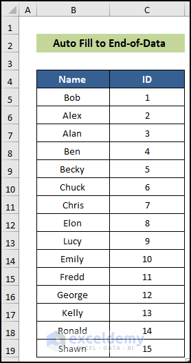
- Excel will autofill the cell automatically.
Read More: How to Apply AutoFill Shortcut in Excel
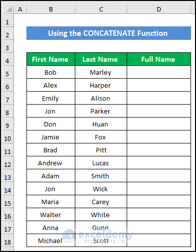
Method 2 – Using the CONCATENATE Function
We have an employee name dataset in separate columns, and we are going to fill the cell of column D.
Steps:
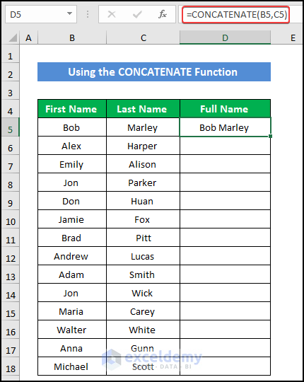
- Select cell D5.
- Use the following formula in the cell.
=CONCATENATE(B5,C5)
- Press Enter.
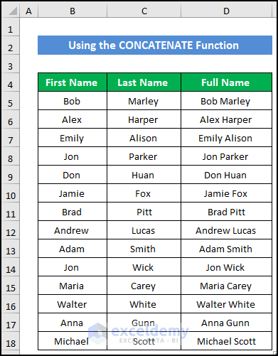
- Double-click on the Fill Handle icon to copy and repeat the formula up to cell D18.
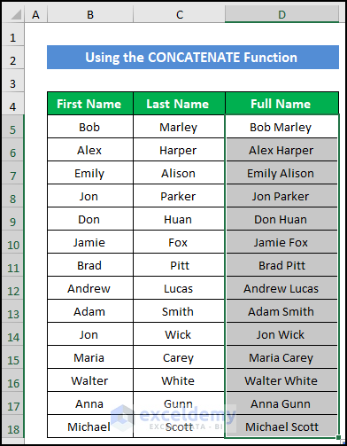
- The formula will autofill the cells of column D.
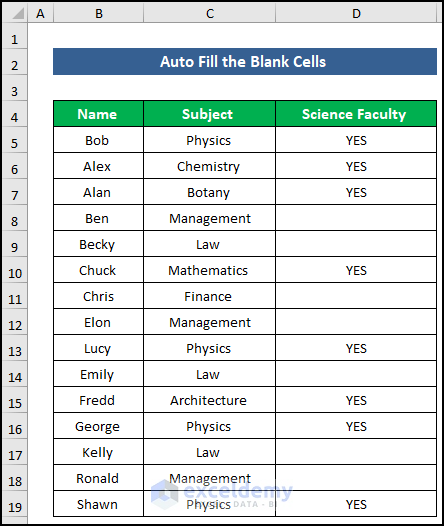
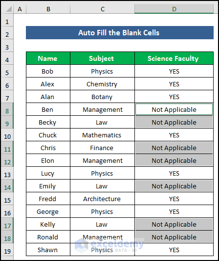
Method 3 – AutoFill Blank Cells Based on Another Cell
We have the “Name” and “Subject” information of some students. Most of them are from the “Science Faculty” (indicated by “YES”). Those who are not from the “Science Faculty” are given blank cells. We are going to auto-fill those cells.
Steps:
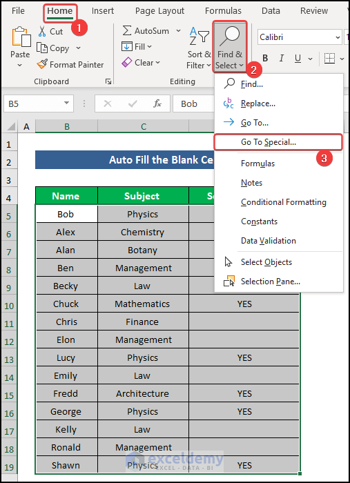
- Select the range of cells B5:D19.
- In the Home tab, click on Find & Select and choose the Go To Special option from the Editing group.
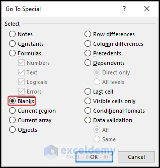
- A small dialog box called Go To Special will appear.
- Select the Blanks option and click OK.
- All the blank cells will be selected.
- Write down your text. We put Not Applicable.
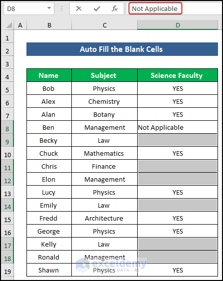
- Press Ctrl + Enter.
- All the blank cells will fill with the desired text.
Read More: Fix: Excel Autofill Not Working
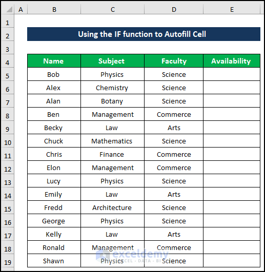
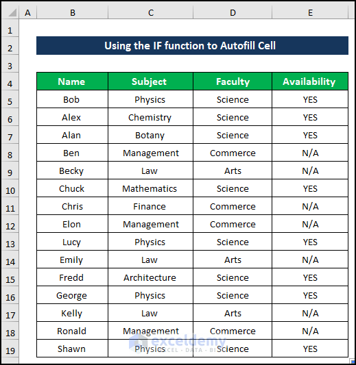
Method 4 – Utilizing the IF function
We have a dataset with the Names of some students, their “Subject”, “Faculty”, and “Availability” of these subjects. We’ll check if the Faculty is Science and apply text in the Availability column.
Steps:
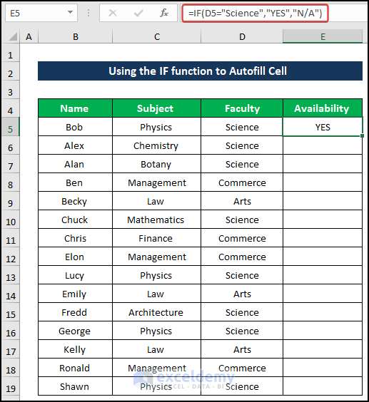
- Select cell E5.
- Use the following formula in the cell.
=IF(D5="Science","YES","N/A")
- Press Enter.
- Double-click on the Fill Handle icon to copy the formula up to cell D19.
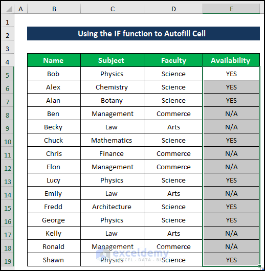
- The formula will autofill the Availability column with results.
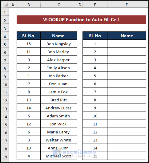
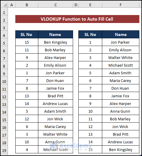
Method 5 – Applying the VLOOKUP function
We have a dataset with a scattered format. We are going to sort this and fill the cells of column F based on column E.
Steps:
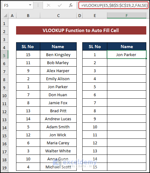
- Select cell F5.
- Use the following formula in the cell:
=VLOOKUP(E5,$B$5:$C$19,2,FALSE)
- Press Enter.
- Double-click on the Fill Handle icon to copy the formula up to cell F19.
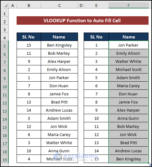
- You will get your desired result.
Download the Practice Workbook
Further Readings
- [Fixed!] Auto Fill Options Not Showing in Excel
- [Fixed!] AutoFill Formula Is Not Working in Excel Table
- How to AutoFill Sequential Letters in Excel
- How to AutoFill from List in Excel
- How to Create a Custom AutoFill List in Excel
- [Solved:] Excel Double Click AutoFill Not Working
<< Go Back to Excel Autofill | Learn Excel
Get FREE Advanced Excel Exercises with Solutions!

Thanks for the info- very helpful!! I also need assistance with: transfering gender and language from one column to another in the same row, but am have trouble finding the formula to do this. Any assistance available for that?
Hi HAZEL,
I am assuming that you want to transfer Gender and Language from one column to another without changing the row position.
In that case, you can insert a new column to the left of the Gender and Language column.
To do so,
● Select the Gender column.
● Then, right-click your mouse to bring the context menu.
● After that, select Insert.
● Excel will add a new column and transfer the Gender and Language column.\
There is another solution to this problem. You can use the OFFSET function. The advantage of this function is that you can transfer any portion of the columns to anywhere in the Excel sheet.
Suppose, I want to transfer B8:C10 to E8:F10. To do so,
● Go to E8 and write down the following formula
=OFFSET(B4,4,0,3,2)
● Then, press ENTER. Excel will move the cells.
● If you use earlier versions of Excel, you have to select E8:F10, then write down the formula and finally press CTRL+SHIFT+ENTER, since the OFFSET function is an array function.
And lastly, you can copy the cells and paste them to transfer columns.
I hope it helps. If it does not satisfy you, please let us know.
Thank you. Have a great day.
Hi there, thank you for this!
If I wanted to only have excel autofill if I had a certain value in a cell, but leave the cell blank if that value wasn’t there, is there a way to do that?
Hello Savannah,
You are most welcome. Yes, you can achieve this easily by using an IF formula. For example:
=IF(A1=”YourValue”, “AutofillText”, “”)
This formula will autofill the cell only when cell A1 contains “YourValue”; otherwise, it’ll remain blank. Let me know if you need further clarification!
Regards
ExcelDemy
Hi there, I’ve been searching the internet for something a little more complex than the basics. I’m hoping someone can help with this matter. I have a column of drivers for our company. Some driver receive 15% of a total, some 20% and some 0%. I am trying to see if I can enter a formula that when I enter drivers name, can another cell have a formula that based on a name it will calculate said percentages, which are based on a total number from another cell. For instance, if A1 = Dan, A2 = $500, can I write a formula to automatically populate A3 at 20% of A2 but if I enter A1 as Bob who receives 15% of A2 can A3 recognize that based on Bob to calculate A2 at 20%?? I hope this isn’t too confusing. Any feedback is helpful!! Thank you!
Hello Nancy,
You can do this with a simple lookup table and a formula.
Create a small table (anywhere) like:
D2:D = Driver Name
E2:E = Percent (enter as 20%, 15%, 0%, etc.)
Then in A3 use either of these:
XLOOKUP (recommended):
=A2*XLOOKUP(A1,$D$2:$D$100,$E$2:$E$100,0)
Or VLOOKUP:
=A2*VLOOKUP(A1,$D$2:$E$100,2,FALSE)
So if A1 = Dan and his rate is 20%, A3 returns 20% of A2. If A1 = Bob and his rate is 15%, it returns 15% of A2. If the name isn’t found, it returns 0 (you can change that behavior if you want).
Regards,
ExcelDemy