In this article, I will show you how to use the Advanced Filter with Wildcard in Excel. As we know, sometimes we need to use the Excel Advanced Filter feature of Excel to filter out strings that are not entirely the same but have some similar pattern. By using Wildcard characters, we are able to filter out all those strings. To know more, read this article carefully.
What Are Wildcard Characters in Excel?
Before jumping into the examples of using the wildcard characters in Advanced Filter in Excel, let’s be familiar with the wildcard characters first. Wildcard characters are special characters used to match texts or take the place of characters in a formula. In Excel, there are three wildcard characters that are frequently used. They are Asterisk(*), Question Mark(?), and Tilde (~). The description and application of these characters are given below.
| WILDCARD CHARACTER | DESCRIPTION | APPLICATION |
|---|---|---|
| Asterisk (*) | It is used to represent any series of characters | B*D will match with BAD, BAKED, BORROWED, etc |
| Question Mark(?) | It is used to represent a single character | S?N will match with SUN, SON. K??L will match with KILL, KAWL |
| Tilde (~) | It is used to use the Wildcard symbols as normal symbols. | BA~*N will match with BA*N
D~?G will match with D?G |
Advanced Filters with Wildcard in Excel: 3 Useful Examples
In this section, we will demonstrate 3 useful examples of using wildcard symbols in Advanced Filter in Excel. We will learn the application of each symbol mentioned above one by one. Let’s explore the first example which will show you the application of the Asterisk symbol.
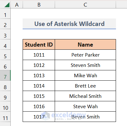
1. Use of Asterisk Wildcard in Advanced Filters
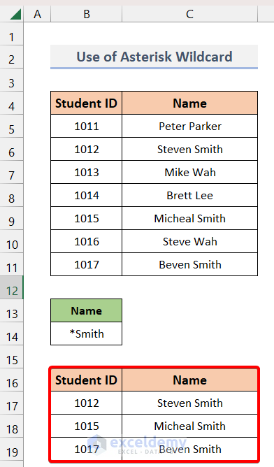
In this example, I have taken a dataset where I have some Students’ Id and their Names. Here, we need to filter out the data whose Name contains Smith in it using Advanced Filter.
To do that, we will have to use the Asterisk(*) wildcard. To know more, follow the steps below.
Steps:
- First, we need to write down the criteria in a separate table under the same column heading as in the actual data table. Hence, I have written the criteria which is *Smith under the heading Name.
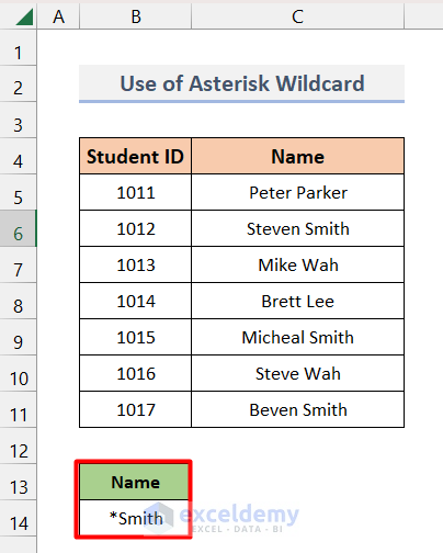
- Here, the criteria *Smith will match any name that contains Smith as the Last Name (Steven Smith, Micheal Smith, and Beven Smith)
- Now, select the whole table(B4:C11), then go to the Data From there, select the Advanced Filter option in the Sort & Filter group.
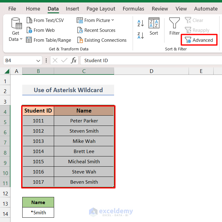
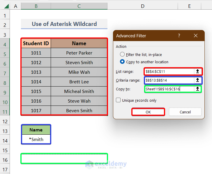
- Consequently, you will see a dialogue box named Advanced Filter. Now, If you want the filtered data to display in another location, then select the Copy to another location. After that, you need to choose the criteria range which is B13:B14, and the location of the filtered data which is B16:C16. Finally, click OK.
- As a result, you will have only the data containing Smith as the last name.
In this way, we can use the Asterisk(*) wildcard for the Advanced Filtering of data in Excel.
2. Application of Question Mark Wildcard in Advanced Filters
In this example, I will use the Question Mark (?) wildcard in Advanced Filter in Excel. For illustration, I have taken another data set containing some Product Ids and Product Names.
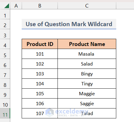
Now, our goal is to find the products that contain ingy at the end with any letter in the beginning (Bingy & Tingy) using the Advanced Filter. To do that, follow the steps below.
Steps:
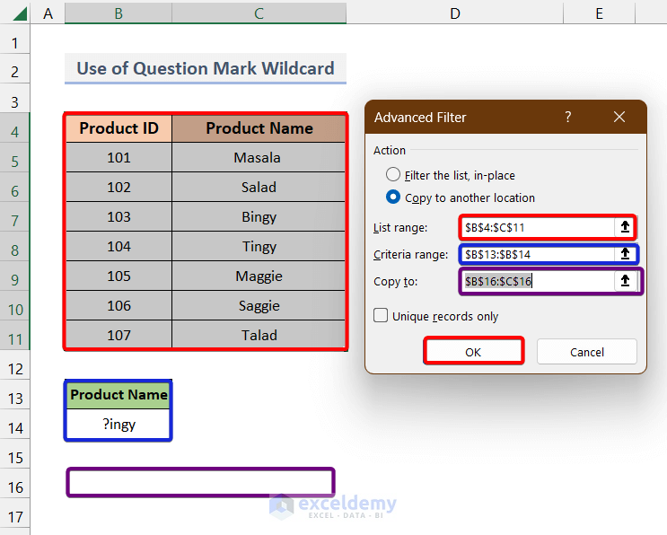
- Like the 1st example, we need to create another table containing the criteria. Hence, we created another table with the heading Product Name and criteria ?ingy.

- Here, the ?ingy will match with any word that has any letter as the first character and then ingy at the last.
- Now, select the whole table(B4:C11), then go to the Data From there, select the Advanced Filter option in the Sort & Filter group.

- Consequently, you will see a dialogue box named Advanced Filter. Now, If you want the filtered data to display in another location, then select the Copy to another location. After that, you need to choose the criteria range which is B13:B14, and the location of the filtered data which is B16:C16. Finally, click OK.
- As a result, you will have only the data containing
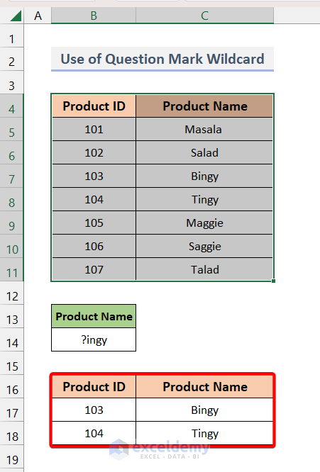
In this way, we can use the Question Mark wildcard in the Advanced Filter in Excel.
3. Utilization of Tilde Wildcard in Advanced Filters
In the final example, we will see the application of the Tilde(~) wildcard in the Advanced Filter. As we have already described, we use this wildcard symbol to match other wildcard symbols(Asterisk and Question Mark) in text. Here, I have taken a data set where we have some texts containing Asterisk(*) and Question Marks.
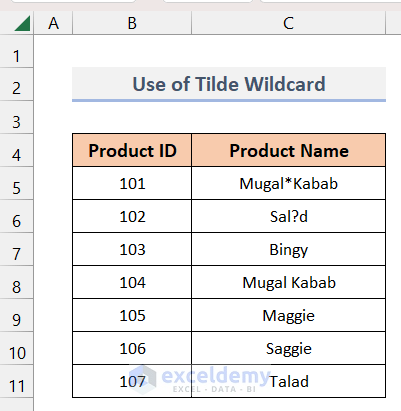
Now, we want to filter the data that contain an Asterisk(*) in the middle. To do that, follow the steps below.
Steps:
- Like the 1st and 2nd examples, create a data table containing criteria which in this case is *~*
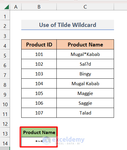
- In this case, the filtered text will have a series of letters at the beginning, so we take one asterisk for it at the beginning of the criteria. Then in the middle, it will have an asterisk(*). Hence, we first gave a tilde sign (~) and then an asterisk(*) so that Excel does not confuse this Asterisk with Wildcard
- Now, use the same procedure to perform Advanced Filter. First, select the whole table(B4:C11), then go to the Data From there, select the Advanced Filter option in the Sort & Filter group.

- As a result, you will see a dialogue box named Advanced Filter. Now, If you want the filtered data to display in another location, then select the Copy to another location. After that, you need to choose the criteria range which is B13:B14, and the location of the filtered data which is B16:C16. Finally, click OK.

- Finally, you will see that the Advanced Filter yields your desired result.

In this way, we can use the Tilde(~) symbol to find other wildcard symbols in a text.
Things to Remember
- In the criteria table, the column header must be the same as in the actual data table.
- If you don’t want to copy the filtered data in another location, you can choose the Filter the list, in-place option in the Advanced Filter Dialogue box.
Download Practice Workbook
Download this practice workbook to exercise while you are reading this article.
Conclusion
That is the end of this article regarding how to use Advanced Filter with Wildcard in Excel. If you find this article helpful, please share this with your friends. Moreover, do let us know if you have any further queries.
<< Go Back to Advanced Filter | Filter in Excel | Learn Excel
Get FREE Advanced Excel Exercises with Solutions!
