How to Delete Unused Rows in Excel (8 Methods)

Dataset Overview

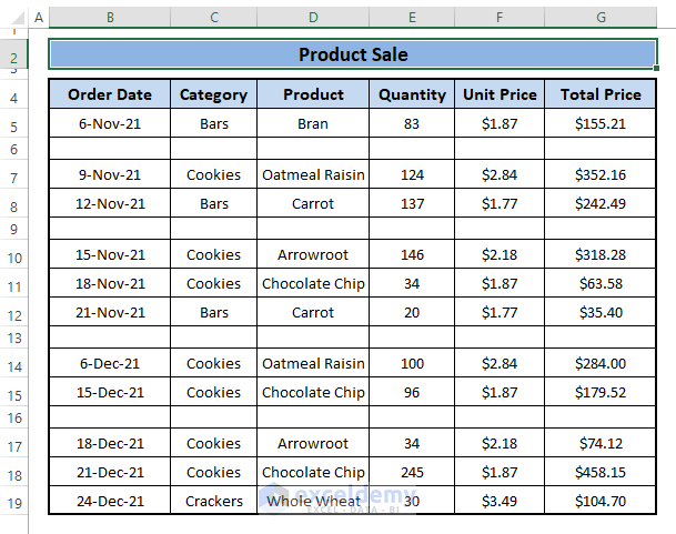
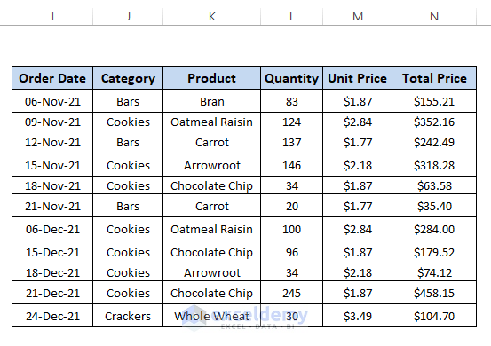
We have a dataset where users input Product Sale data. Somehow users leave unused or blank rows while entering data in the dataset as can be seen in the below image.

Method 1 – Using the Context Menu

If you have a small dataset with only a few unused rows, follow these steps:

• Press and hold the CTRL key.

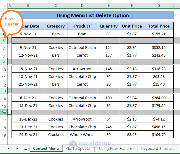
• Click on the blank rows you want to delete (you can select entire rows by clicking on the row headers).

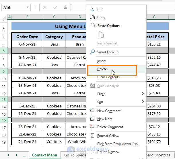
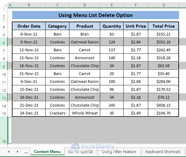
• Right-click on the selected rows and choose Delete from the Context Menu. This will remove the unused rows.

Method 2 – Go To Special Feature

For larger datasets with numerous blank rows, Excel’s Go To Special feature is helpful:

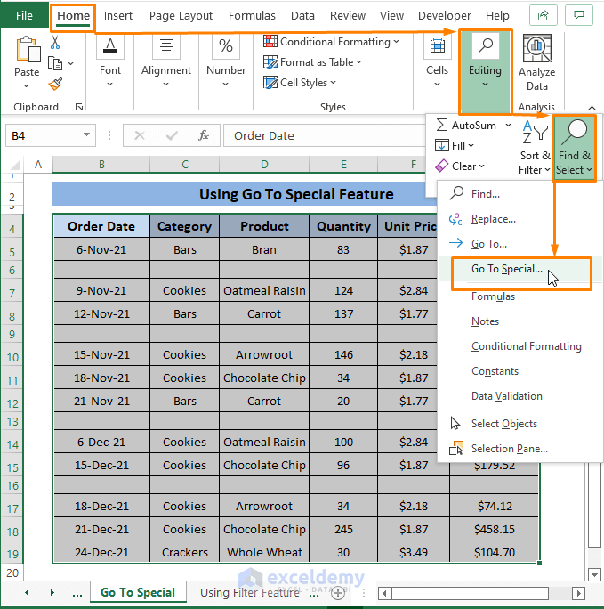
• Go to the Home tab.
• In the Editing section, click on Find & Select and choose Go To Special.

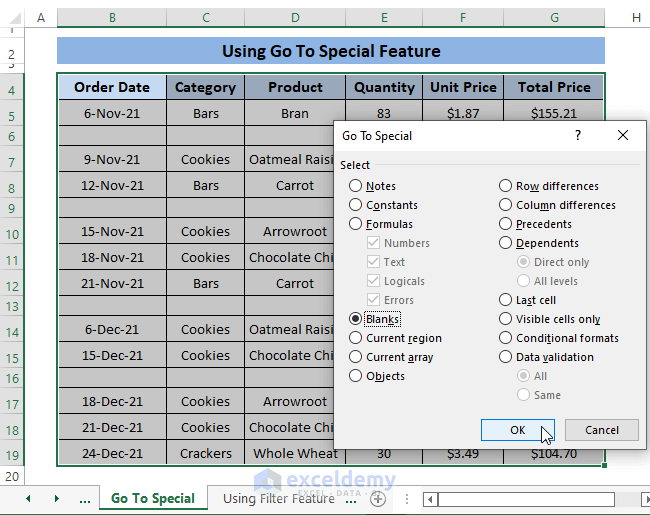
• In the dialog box, select Blanks and click OK.  This selects all the blank rows in the dataset.

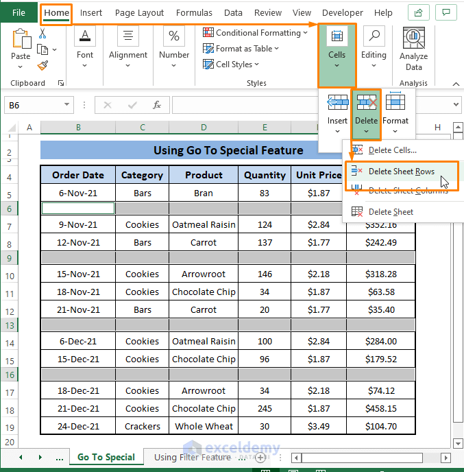
• Go back to the Home tab, choose Delete from the Cells section, and click Delete Sheet Rows.

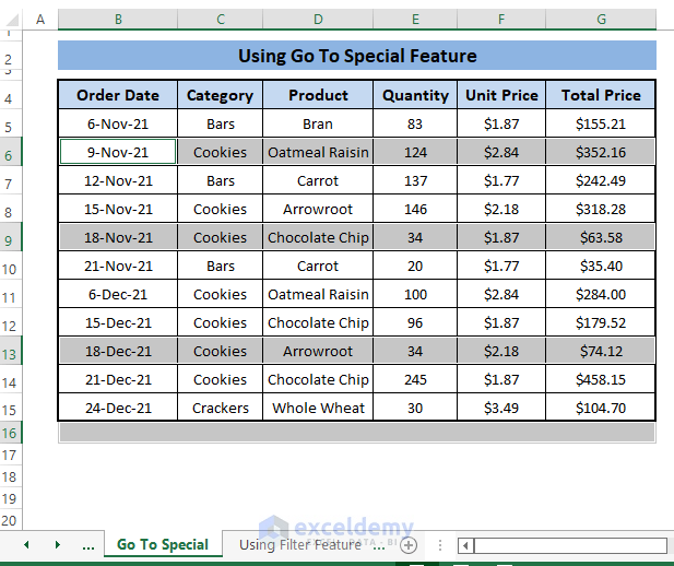
Your dataset will no longer contain unused rows.

Method 3 – Using the Filter Feature

Excel’s Filter feature can also help:

• Select the range containing your data.
• Go to the Data tab and click on Filter in the Sort & Filter section.

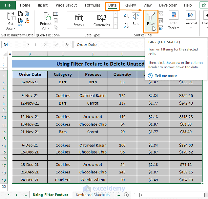
• Filter icons will appear in the column headers.
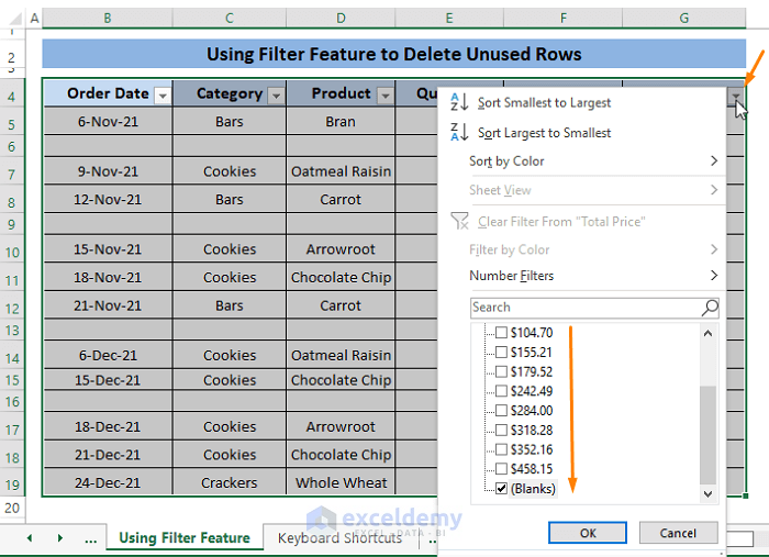
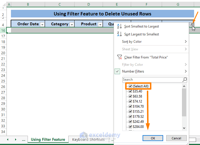
• Click on any filter icon and select all entries except Blanks.
• Click OK to display only the blank rows.

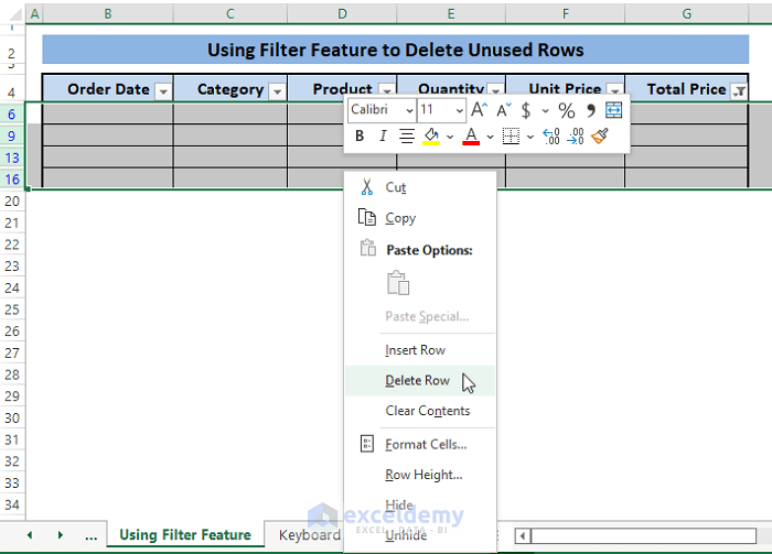
• Select these unused rows by dragging the mouse cursor along the row headers.
• Right-click and choose Delete Row from the Context Menu.

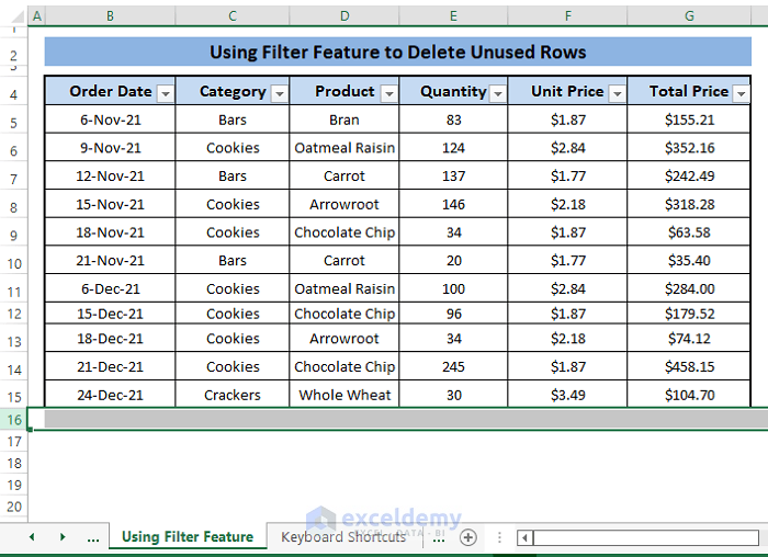
The below image shows the result.

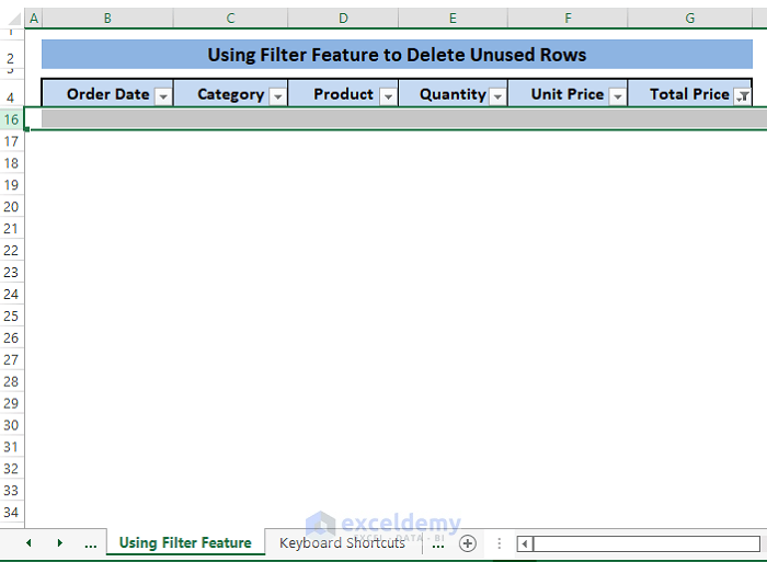
• Click on the Filter icon in any column header and Check the Select All option.
• Click OK.

• All the rows, except unused ones will appear.

Read More: How to Delete Filtered Rows in Excel?

Method 4 – Using Keyboard Shortcuts to Hide Rows 

Sometimes we don’t want to delete unused rows outside the dataset range. Instead, we can hide them to keep our view tidy:

• Place the cursor on any cell outside the range.
• Press CTRL+SHIFT+Down Arrow to select all rows up to row number 1048576 (the last row in an Excel worksheet).

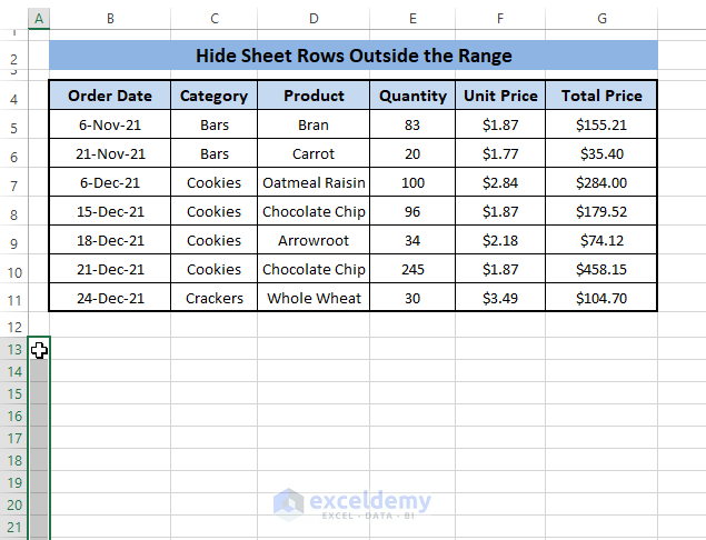
• Press SHIFT+SPACE to select all corresponding columns.

• Right-click on any selected cell and choose Hide from the Context Menu.

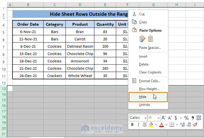
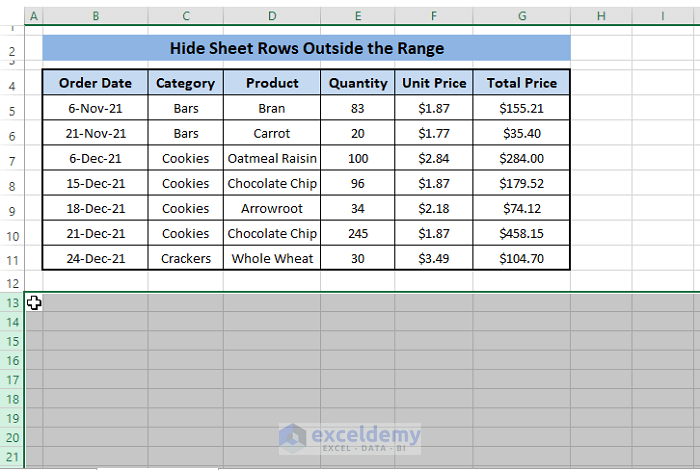
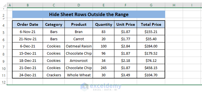
This hides the unused rows below the dataset.

Read More: How to Delete Hidden Rows in Excel?

Method 5 – Excel Sorting Feature

Excel’s sorting feature can help push unused rows to the bottom of the dataset:

• Select the entire dataset.
• Go to the Data tab and click on Ascending (A to Z) or Descending (Z to A) sorting in the Sort & Filter section.

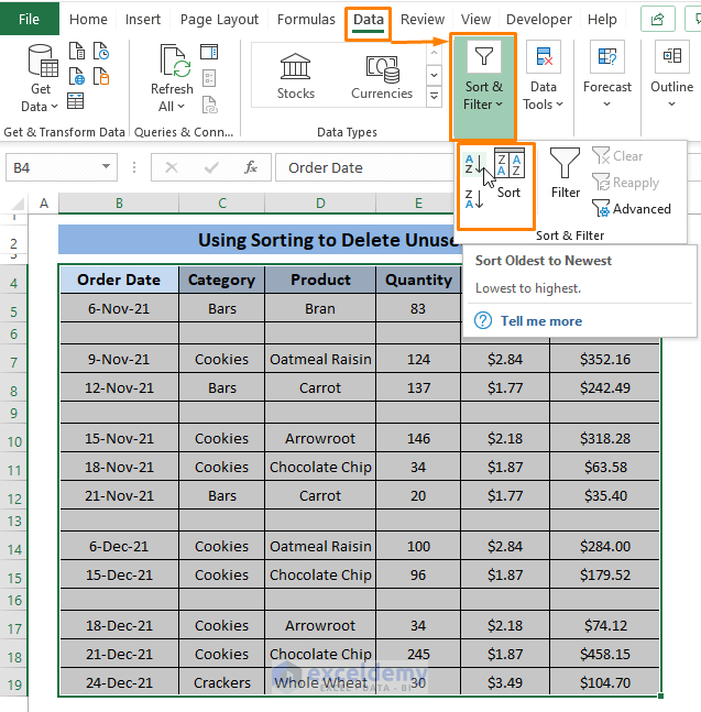
• This reorders the rows, placing unused ones at the bottom.
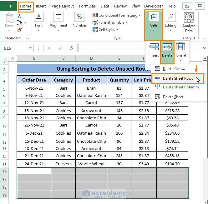
• Go to the Home tab, select Delete from the Cells section, and click Delete Sheet Rows.

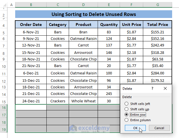
You can also use this alternative way to delete the unused blank rows:

• Right-Click (CTRL+- can also be used) on the selected Blank rows, the Context Menu appears, select Delete.

• A Delete dialog box will pop up. Click on Entire row. Click OK.

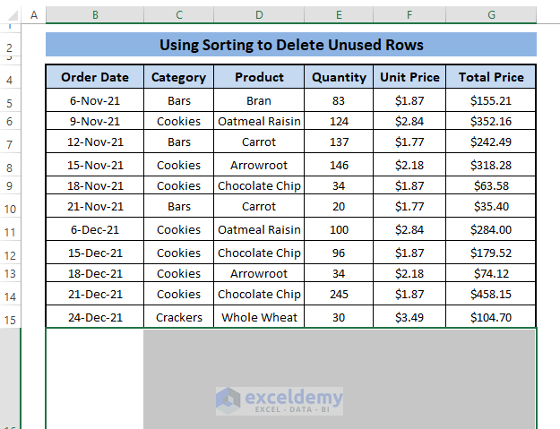
Following these steps to delete the unused rows as shown in the below picture:

Method 6 – Using the Find Feature

Similar to filtering or sorting, the Find feature can locate all blank cells in a dataset:

• Highlight the entire dataset.
• Go to the Home tab, click on Find & Select in the Editing section, and choose Find.

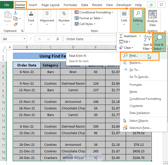
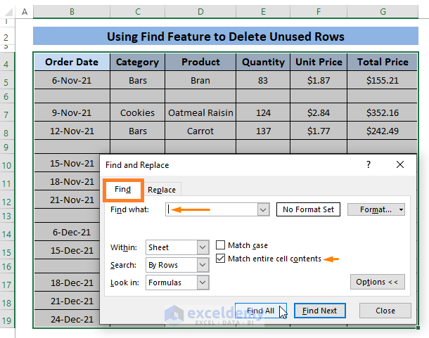
• In the Find and Replace dialog box, leave the Find What option blank and check Match entire cell contents.
• Click Find All to display all blank rows.

• Press CTRL+A to select all unused rows.

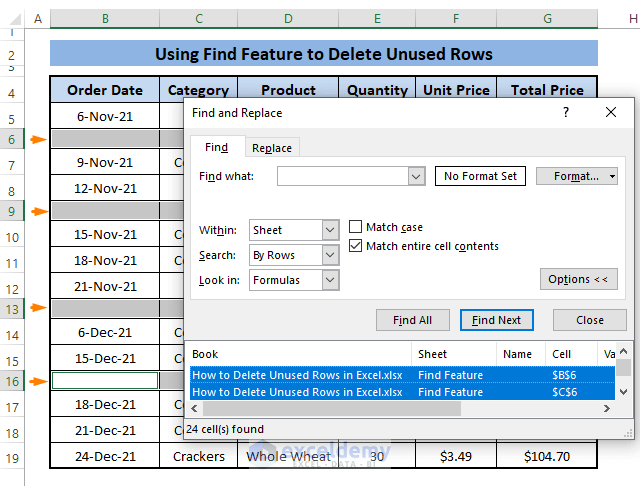
• Right-click and choose Delete from the Context Menu.

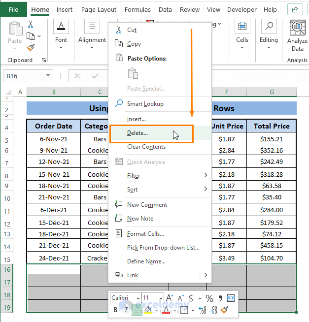
• In the delete dialog box, select Entire row and click OK.

Executing all the sequential steps deletes all the unused rows as depicted in the following picture:

Method 7 – Using the Filter Function

The FILTER function is available in Microsoft Excel 365 and allows you to filter a range of data based on a given criterion:

• The syntax is:

Here’s how it works:

• • array: Specify the range you want to filter (e.g., B5:G19).
  • include: A Boolean array that acts as the filtering criterion (e.g., E5:E19>10).
  • [if_empty]: Optional return value when no matches are found.

We can use the FILTER function to delete the unused rows in a dataset.

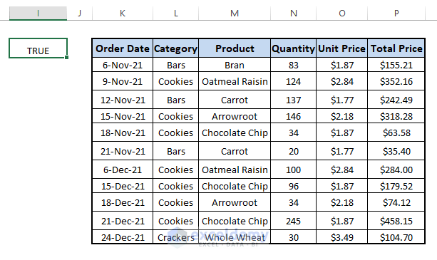
• In an adjacent blank cell (e.g., I5), enter the formula:

• Press Enter.

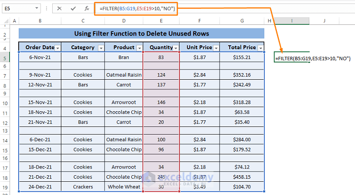
• This will create a dataset without blank rows, as shown below:

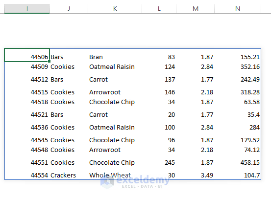After formatting and inserting column headers the whole dataset looks like the below screenshot without unused rows.

Method 8 – Using the Advanced Filter Feature

Similar to the FILTER function, the Advanced Filter feature allows you to delete unused rows by copying the dataset to another location without blank rows:

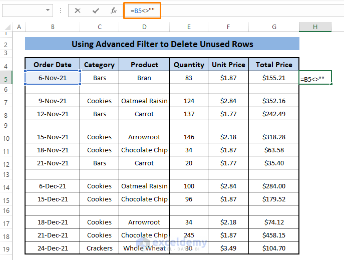
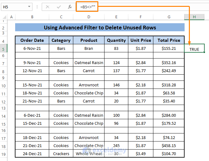
• Set a criterion (e.g., in cell H5), and enter:

The criterion says it’ll match entries before or after the cell reference B5 (i.e., Order Date 6 Nov, 21).

• Select the entire dataset.
• Go to the Data tab, choose Advanced Filter from the Sort & Filter section.

• In the Advanced Filter dialog box:
  • The list range (B4:G19) will be automatically selected.
  • Specify the criteria range (H4:H5).
  • Choose to copy the filtered data to cell I5.

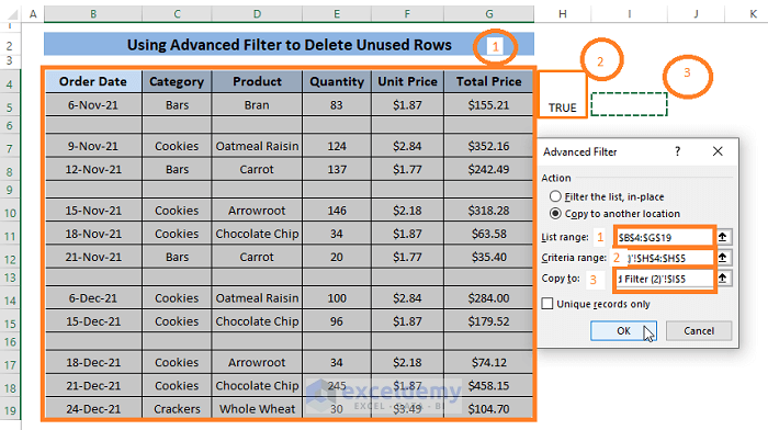
• Click OK to get a dataset without unused rows, as shown below:

Download Excel Workbook

You can download the practice workbook from here:

Things to Remember

Be mindful of your data type when choosing a method to delete unused rows.

Some methods may inadvertently remove necessary information, so select the approach that best suits your dataset.

Related Articles

• How to Find and Delete Rows in Excel
• How to Delete Multiple Rows in Excel Using Formula?
• How to Delete Multiple Rows in Excel with Condition?
• How to Delete Rows in Excel That Go on Forever?
• How to Delete Infinite Rows in Excel?
• How to Remove Rows Containing Identical Transactions in Excel?

<< Go Back to Delete Rows | Rows in Excel | Learn Excel