How to Delete Blank Rows in Excel?

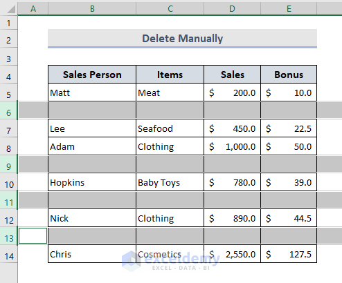
Method 1 – Delete a Couple of Blank Rows Manually

Press & hold the Ctrl key and select the blank rows.

Right-click > Go to the context menu > Click on the Delete command.

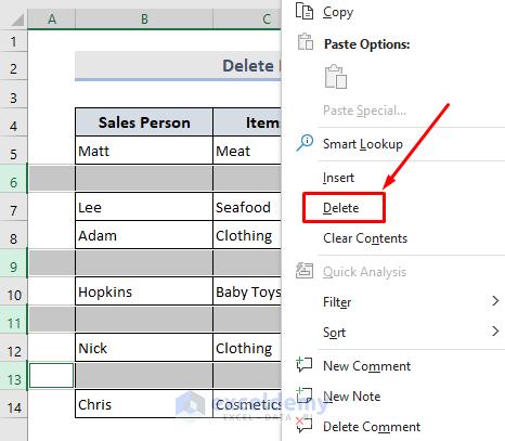
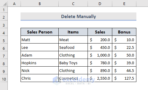
The Keyboard Shortcut for the Delete Command is: Ctrl + –

The selected empty rows will be deleted.

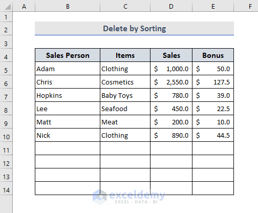
Method 2 – Use Excel Sort Command

Go to the Data tab > The Sort and Filter group.
Click on Sort Smallest to Largest or Sort Largest to Smallest.

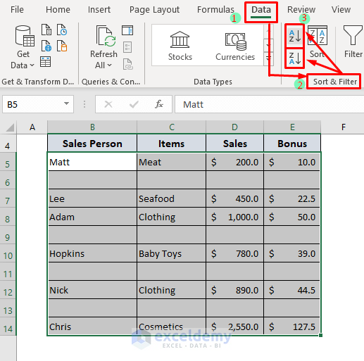
The blank rows are sorted out to the bottom as shown in the following image.

Remember:
If the dataset has a column for serial numbers, select the Sort Smallest to Largest option so that the serial numbers don’t alter.

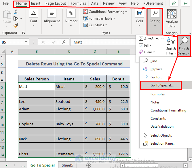
Method 3 – Use Go To Special Command

Select any column or the whole dataset.

To select a column/ the whole dataset, select the first cell, hold the Shift key, and select the last cell.

Go to the Home tab > The Editing group.
Go to the Find & Select drop-down menu > The Go To Special command.

The Go To Special dialog box will open.

Shortcut: Press Ctrl + G > Go To dialog box will open > Press Special.

Select the Blanks radio button > Press OK.

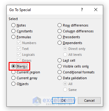
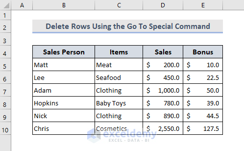
The following image shows that the blank rows along with the blank cells are selected.

To delete the selected rows.

Press Ctrl + –.
The Delete dialog box will open.

Select the Entire row radio button > Press OK.

Method 4 – Utilize Excel Find Command

Go to the Home tab > The Editing group.
The Find & Select drop-down > The Find Command.

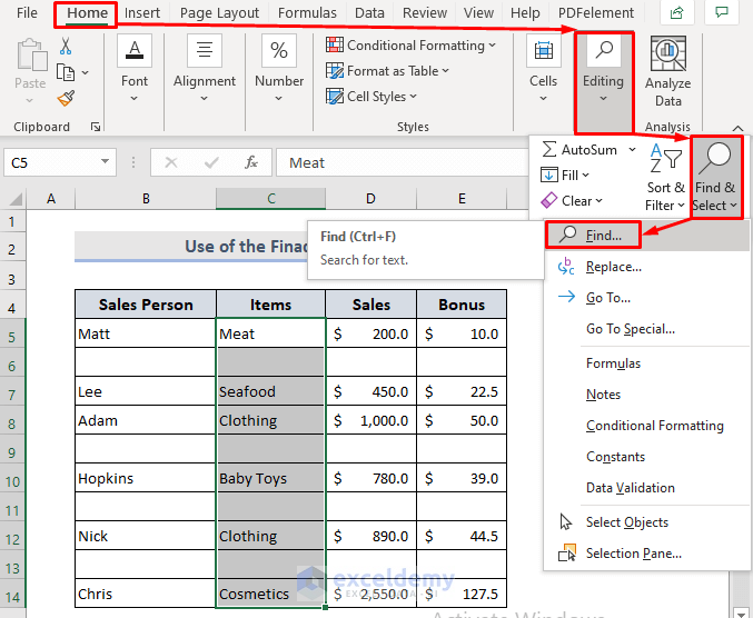
A dialog box named Find and Replace will appear.

We can also get to Find and Replace by pressing Ctrl + H on the keyboard.

Go to Find.
Keep the Find what box blank.
Search Within the Sheet.
Search By Rows.
Look in the Values.
Mark the Match entire cell contents checkbox.
Press Find All.

All 4 blank rows are shown in the pop-up box.

Select all by pressing Ctrl + A.
Press Close.

Delete all by following any methods shown above..

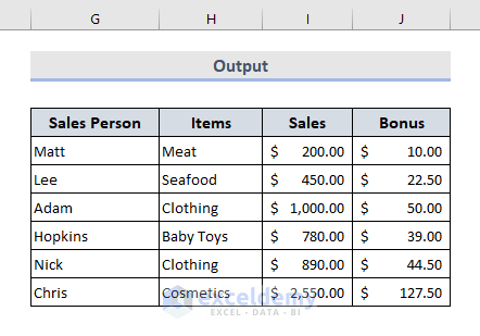
The output will be as shown in the image below.

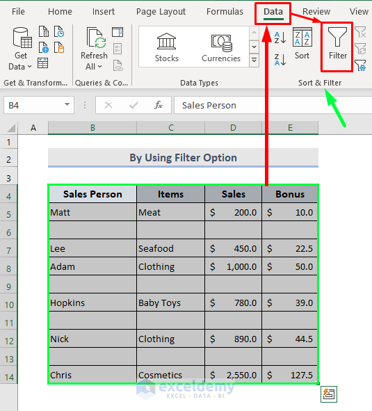
Method 5 – Use Excel AutoFilter Feature

Select the entire range of data including the headers, B4:E14.
Go to the Data tab > The Sort & Filter group > Turn on the Filter option by clicking on it.

The keyboard shortcut for turning on the Filter option is: Ctrl+Shift+L

Click on any of the showing all icons of the headers.
Unselect all > Select only Blanks.
Press OK.

All the rows which has any content will disappear. Only the blank rows will be visible.

Delete the blank rows by following the steps described in Method 1.

Though we have deleted the blank rows, the result shows the dataset with the missing data. Recover the rows with the data.

Click on any of the showing all icons of the headers of the dataset.
Select All > Press OK.

We have got back our original dataset which is now without any blank rows. The next task is to convert it to an unfiltered form.

Click on a random cell in the dataset and go to the Data tab.
Go to the Sort & Filter group > Click on the Filter command.

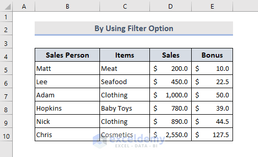
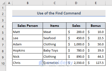
An Alternative Way to Use the Filter Option:

Apply the Filter command on the dataset.
Click on any of the showing all icons of the headers.

Unmark the (Blanks) checkbox > Press OK.

Keep the Filter option ON.

Remember:
It should be noted that if we turn off the Filter option, the blank rows will appear.

Related Content: How to Delete Rows in Excel with Specific Text

Method 6 – Use Excel Advanced Filter Command

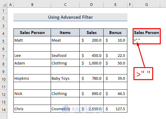
Create a new data column in Cell G4 with a header named Sales Person.
Enter >”” in Cell G5.

Go to the Data tab > Go to the Sort & Filter group > Click on the Advanced option.

The advanced filter dialog box will open up.

Click on the “Filter the list, in-place” radio button.
Select the “List range” by selecting the entire dataset B4:E14.

Select the “Criteria range” by selecting the range G4:G5.

The Advanced Filter dialog box will look as shown in the following image.

Press OK.

The blue & non-sequential row numbers 5,7,8,10,12 and 14 indicate that the blank rows are still there though not displayed. Double click between the blue rows to display it in the dataset.

Method 7 – Use Several Excel Formulas to Delete Blank Rows

7.1 Use Excel FILTER Function

Copy the header names and paste them in a new location (here, in Cell G4) with formatting.
Enter the following formula using the FILTER function in Cell G5:

=FILTER(B5:E14,(B5:B14<>"")*(C5:C14<>"")*(D5:D14<>"")*(E5:E14<>""))

Press Enter.

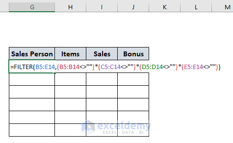
All the blank rows will be removed.

How Does the Formula Work?

We are looking for blank rows to delete, each of the blank rows’ cells will be blank. We have designed criteria to find the blank cells first. Using Boolean logic, we have deleted the blank cells.

⮞ E5:E14<>””
The NOT operator with an empty string “” means Not Empty. In each cell in the range E5:E14, the result will be an array as follows:
Output: {TRUE;FALSE;TRUE;TRUE;FALSE;TRUE;FALSE;TRUE;FALSE;TRUE}

⮞ Similarly, for D5:D14<>””, C5:C14<>”” and B5:B14<>””, the results will be:
D5:D14<>””= {TRUE;FALSE;TRUE;TRUE;FALSE;TRUE;FALSE;TRUE;FALSE;TRUE}
C5:C14<>””= {TRUE;FALSE;TRUE;TRUE;FALSE;TRUE;FALSE;TRUE;FALSE;TRUE}
B5:B14<>””= {TRUE;FALSE;TRUE;TRUE;FALSE;TRUE;FALSE;TRUE;FALSE;TRUE}

⮞ (B5:B14<>””)*(C5:C14<>””)*(D5:D14<>””)*(E5:E14<>””)
Following the rules of Boolean logic, this returns the following array.
Output: {1;0;1;1;0;1;0;1;0;1}

⮞ FILTER(B5:E14,(B5:B14<>””)*(C5:C14<>””)*(D5:D14<>””)*(E5:E14<>””))
The FILTER function returns the output from the array B5:B14, which matches the criteria.=
Output: {“Matt”,”Meat”,200,10;”Lee”,”Seafood”,450,22.5;”Adam”,”Clothing”,1000,50;”Hopkins”,”Baby Toys”,780,39;”Nick”,”Clothing”,890,44.5;”Chris”,”Cosmetics”,2550,127.5}

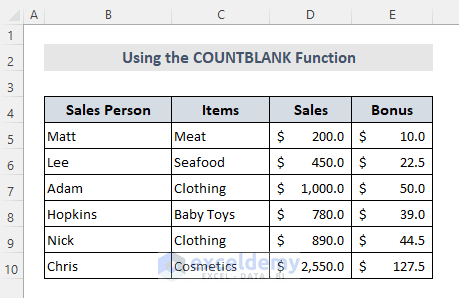
7.2 Use COUNTBLANK Function

The COUNTBLANK function returns the number of blank cells in a specified range. Though it deals with blank cells, we can utilize the function for our cause too. Let’s see then.

Steps:

Add a column named “Blanks” to the right side of the dataset.
Enter the formula ⏩ =COUNTBLANK(B5:E5) ➤ in Cell F5.

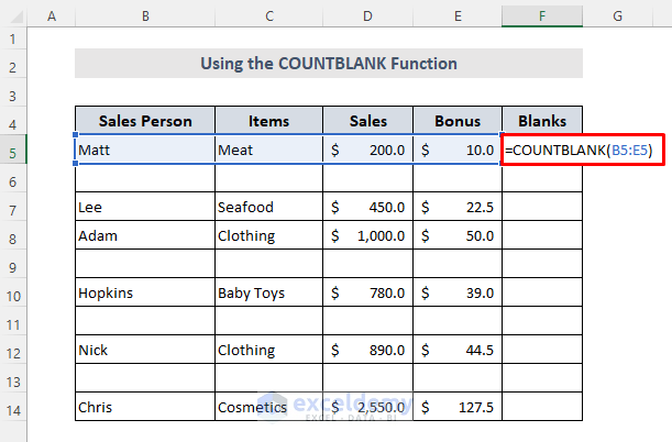
Drag the Fill handle icon over the range F6:F14.

Go to the Data tab > Go to the Sort & Filter group.
Turn on the Filter option.

Keyboard shortcut for Filter option: Ctrl+Shift+L

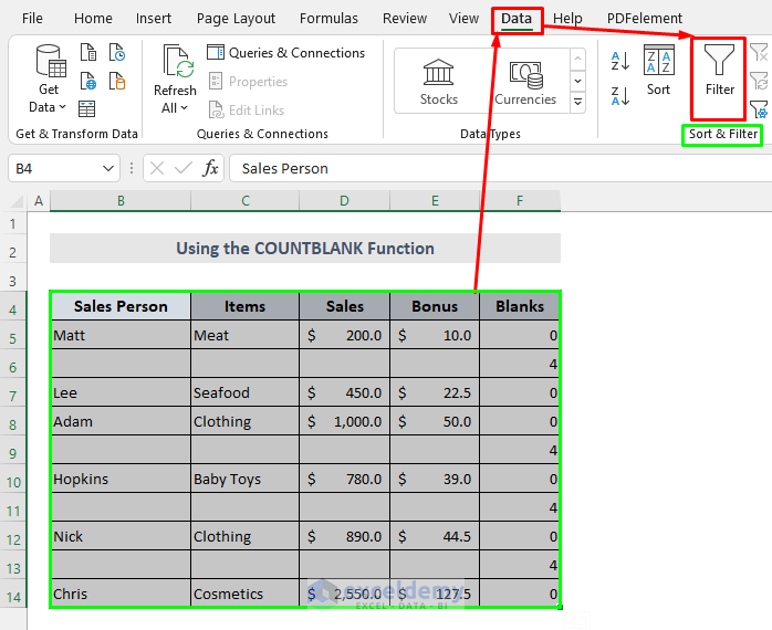
Click on any of the showing all icons at the headers of the dataset.
Unselect all > Select only 4.
Press OK.

Delete the existing rows by using any technique described in method 1.
Go to the Data tab and click on the Filter option and turn it off.

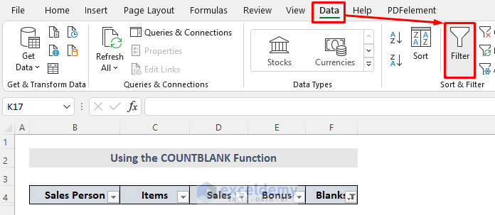
After turning the Filter option off, the dataset will look like the following image.

Delete column F by selecting the column and selecting the Delete command from the context menu.

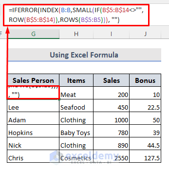
7.3 Combine INDEX, SMALL, ROW, and ROWS Functions

Copy the headers of the dataset and paste in another location (Cell G4).
Enter the following formula in Cell G5 and pressEnter.

=IFERROR(INDEX(B:B,SMALL(IF(B$5:B$14<>"",ROW(B$5:B$14)),ROWS(B$5:B5))), "")

If you don’t have MS Excel 365, press Ctrl+Shift+Enter.

Drag the fill handle icon to the right and bottom end of the dataset.

How Does the Formula Work?

⮞ ROWS(B$5:B5)
ROWS function returns the number of rows in the range B$5:B5.
Output: 1.

⮞ ROW(B$5:B$14)
The ROW function returns the row number of the range B$5:B$14.
Output: {5;6;7;8;9;10;11;12;13;14}

⮞ B$5:B$14<>””
Output: {TRUE;FALSE;TRUE;TRUE;FALSE;TRUE;FALSE;TRUE;FALSE;TRUE}

⮞ IF(B$5:B$14<>””, ROW(B$5:B$14))
The IF function checks the range B$5:B$14 whether it satisfies the condition, and returns the following.
Output: {5;FALSE;7;8;FALSE;10;FALSE;12;FALSE;14}

⮞ SMALL(IF(B$5:B$14<>””, ROW(B$5:B$14)),ROWS(B$5:B5))
The SMALL function determines the smallest value of the above array.
Output: {5}

⮞ IFERROR(INDEX(B:B,SMALL(IF(B$5:B$14<>””, ROW(B$5:B$14)),ROWS(B$5:B5))), “”)
Finally, the INDEX function returns the value from the B:B range and 5th row, as called by the SMALL function. The IFERROR function is just to keep the output fresh from Excel error values.
Output: {Matt}

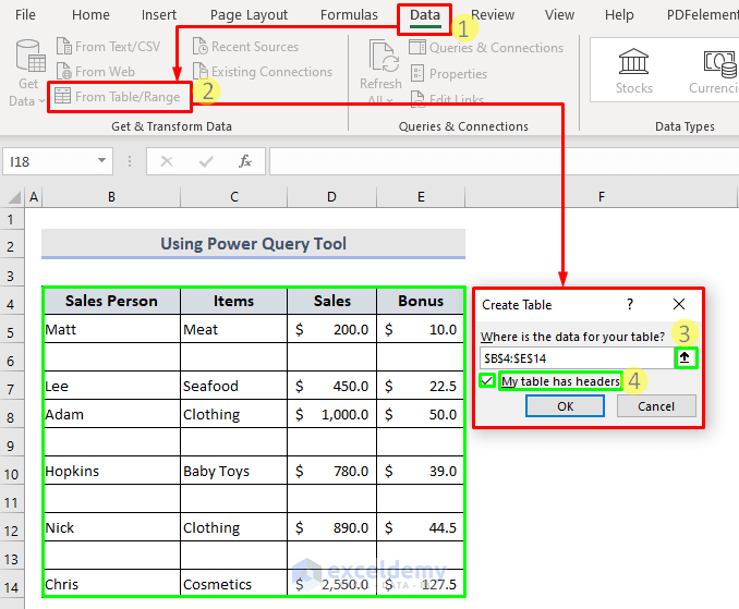
Method 8 – Use the Excel Power Query Tool to Delete All Blank Rows

Go to the Data tab > “Get & Transform Data” group > Select the “From Table/Range” option.
A “Create Table” dialog box will open.

Select the entire dataset B4:E14.
Press OK.

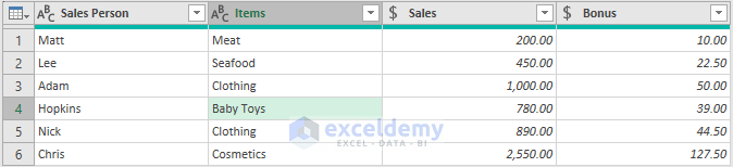
The “Power Query Editor” window will open.

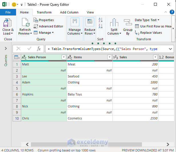
Go to the Home tab > Reduce Rows drop-down menu
Remove Rows drop-down > Remove Blank Rows.

The blank rows will be deleted.

Go to File > Select Coles & Load To option.

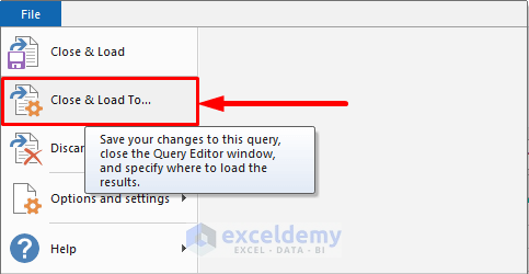
The Import Data dialog box will open.

Choose the Table radio button.
Choose the Existing worksheet radio button
Select your desired placement of the output, Cell B16 > Press OK.

Converting the Dataset to Range Form:

Go to the Table Design tab > the Tools group > Select Convert to Range.
Press OK.

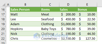
The Sales and Bonus column data are in the General number type. You can change the number type.

1. Select the two columns.

2. Go to the Home tab > Number group > Select Accounting Number Format.

Download Practice Workbook

Delete Blank Rows.xlsx

<< Go Back to Delete Rows | Rows in Excel | Learn Excel

Get FREE Advanced Excel Exercises with Solutions!