Method 1 – Delete Rows Based on Another List by Applying the Excel COUNTIF Function and Sort Option
Steps:
- Type the below formula in Cell D5 (on the helper column) at first.
=COUNTIF($F$5:$F$8,B5)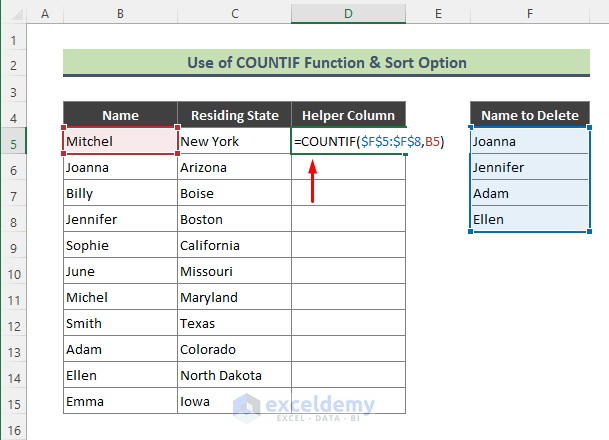
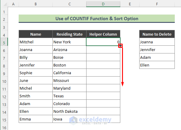
- Hit Enter, the formula will return the below result. Use the Fill Handle (+) to copy the formula over the range D6:D15.
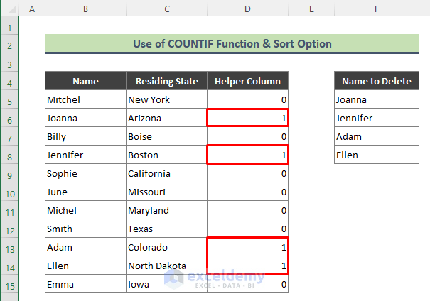
- The following will be the output. The COUNTIF function returns ‘1’ if any of the employee names from the range B5:B15 matches the list F5:F8.
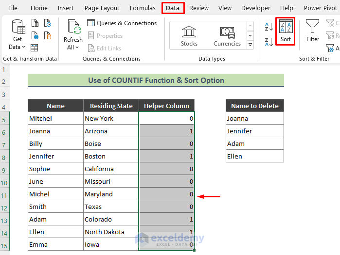
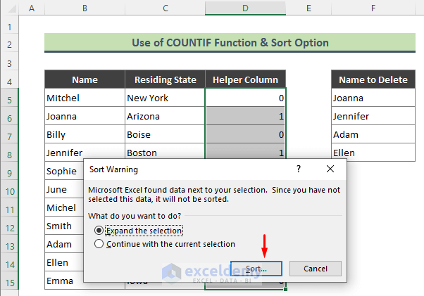
- Sort the data that matches to names to be deleted. Select the helper column and go to Data > Sort.
- The Sort Warning dialog will appear; click Sort.
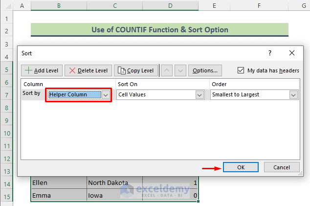
- The Sort dialog will show up. Ensure the below fields are the same as the following screenshot and click OK.
- Clicking OK, all the matched rows will be sorted as below.
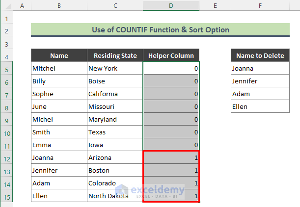
- Select all the rows that contain 1 in the helper column by pressing the Ctrl key from the keyboard. Right-click on the selection and press Delete.

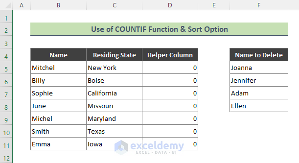
- You will get the below result.
Method 2 – Apply Filter Option with Combination of IF, ISERROR, VLOOKUP Functions to Remove Rows Based on Another List
Steps:
- Add an extra helper column to the main dataset (B4:C15), and type the below formula in Cell D5 (Sheet1) and press Enter.
=IF(ISERROR(VLOOKUP(B5,Sheet2!B:B,1,FALSE)),"Keep","Delete")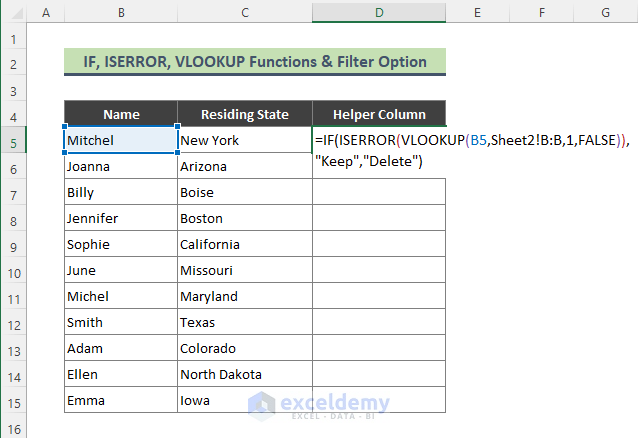
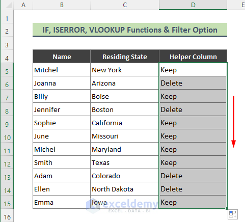
- Get the below result. I have used the Fill Handle to copy the formula to the rest of the cells. The formula used above put ‘Delete’ against employee names matching the list in Sheet2.
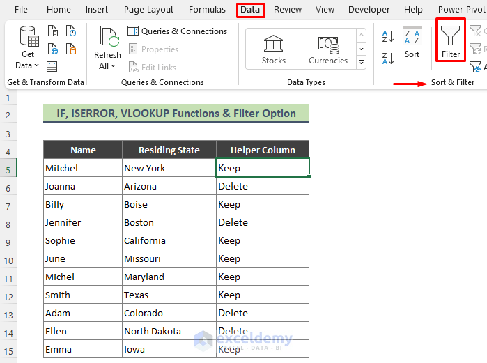
- Filter all the rows that contain ‘Delete’ from the helper column. Go to Data > Filter.
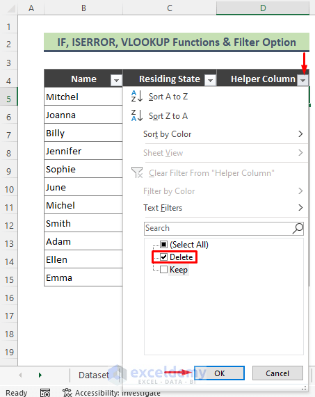
- The drop-down icon to apply the filter will appear. Click the drop-down icon of the helper column and filter the data only for ‘Delete’. Press OK.
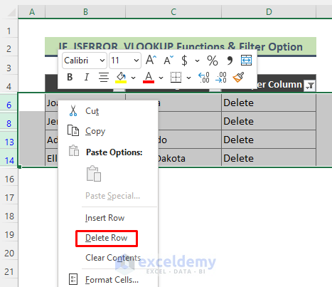
- Press OK, rows that contain ‘Delete’ will be filtered; now, select all the rows and right-click on them. Click Delete Row.
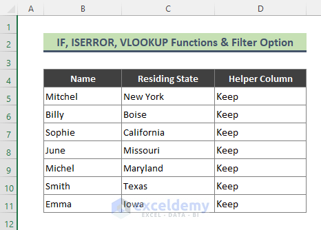
- All the rows will be deleted. Press Ctrl + Shift + L to withdraw the Filter. You will get the below result.
How Does the Formula Work?
- VLOOKUP(B5,Sheet2!B:B,1,FALSE)
Here the VLOOKUP function looks for names of Cell B5 (Sheet1) in column B:B (Sheet2) and return:
{N/A}
The formula returns the employee name if it is found in the list to be removed.
- ISERROR(VLOOKUP(B5,Sheet2!B:B,1,FALSE))
The ISERROR function converts the result of the VLOOKUP formula to TRUE/FALSE. For Cell D5, this part of the formula returns:
{TRUE}
- IF(ISERROR(VLOOKUP(B5,Sheet2!B:B,1,FALSE)),”Keep”,”Delete”)
The IF function returns Keep if the result of the ISERROR formula is TRUE, returns Delete. For Cell D5, the above formula returns:
{Keep}
Methods 3 – Combine Excel ISNA, MATCH & IF Functions to Remove Rows Based on Another List
Steps:
- Type the following formula in Cell D5 and hit Enter.
=IF(ISNA(MATCH(B5,SheetY!B:B, 0)),"Keep", "Delete")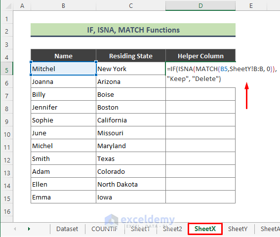
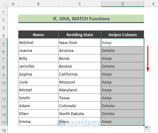
- Use the Fill Handle to copy the formula to the range over D6:D15.
- Apply SORT or FILTER to the above result and thus remove the rows that contain ‘Delete’ in the helper column. (See Method 1 or Method 2 for details).
How Does the Formula Work?
- MATCH(B5,SheetY!B:B, 0)
The MATCH function matches the value in Cell B5 (SheetX) in column B:B (SheetY) and returns the row number if the names are matched. It returns the #N/A error. The formula returns the following for Cell D5:
{#N/A}
- ISNA(MATCH(B5,SheetY!B:B, 0))
Later MATCH formula is passed through the ISNA function to return TRUE/FALSE depending on the match/mismatch. For Cell D5, the formula returns:
{TRUE}
- IF(ISNA(MATCH(B5,SheetY!B:B, 0)),”Keep”, “Delete”)
The IF function returns Keep if the result of the ISNA formula is TRUE, it returns FALSE otherwise. The following is returned for Cell D5:
{Keep}
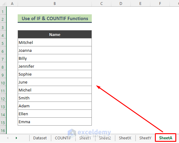
Method 4 – Use IF and COUNTIF Functions to Delete Excel Rows Dependent on Another List
You can combine the COUNTIF function along with the IF function to remove rows that contain data from another list. We use three Excel worksheets to perform the task. Say your dataset is in SheetA.
The list to be removed is in SheetB.
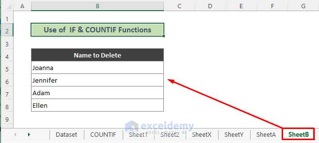
Let’s follow the below steps to complete the operation.
Steps:
- Go to a new worksheet (SheetC). Type the below formula in Cell B4 of SheetC.
=IF(COUNTIF(SheetA!$B:$B,SheetB!B5)>0,"",SheetA!B5)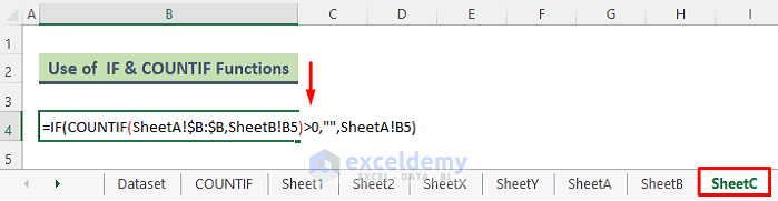
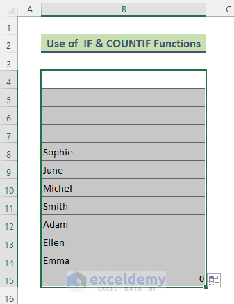
- Drag down the ‘+’ sign until you receive 0 in return.
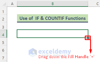
- We can see that the 4 blank rows out of 12 rows. This is because the names in these 4 rows match the list B5:B8 of SheetB.
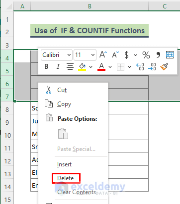
- You can delete all the blank rows from the above output in SheetC by simply right-clicking on the blank rows.
How Does the Formula Work?
- COUNTIF(SheetA!$B:$B,SheetB!B5)
The COUNTIF function looks for values of Cell B5 (SheetB) in column B:B (SheetA) and returns the count. The first entry of Sheet C, the formula returns:
{1}
- IF(COUNTIF(SheetA!$B:$B,SheetB!B5)>0,””,SheetA!B5)
The IF function returns blank (“ ”) if the result of the COUNTIF formula is greater than 0, otherwise the formula returns the employee name from SheetA. The above formula returns the below result for Cell B5 (SheetC).
{ }
Method 5 – VBA to Delete Excel Rows Dependent on Another List
Steps:
- Right-click on Sheet7 and click on View Code to bring up the VBA window.
- Type the below code in the Module and run the code using the F5 key or pressing the Run Sub/UserForm icon (see the screenshot).
Sub DelRows_TwoLists()

Dim iList As Integer
Dim Ctr As Integer
Application.ScreenUpdating = False
iList = Sheets("sheet7").Range("A1:A12").Rows.Count
For Each x In Sheets("Sheet8").Range("A1:A5")
For Ctr = 1 To iList
If x.Value = Sheets("Sheet7").Cells(Ctr, 1).Value Then
Sheets("Sheet7").Cells(Ctr, 1).EntireRow.Delete xlShiftUp
Ctr = Ctr + 1
End If
Next Ctr
Next
Application.ScreenUpdating = True
MsgBox "Complete!"

End Sub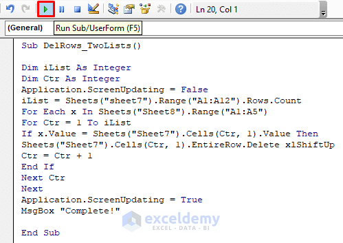
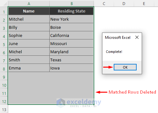
- Rows matching the list of Sheet8 will be removed. The message box below will appear. Click OK to end the process.
Download Practice Workbook
You can download the practice workbook that we have used to prepare this article.
Related Articles
- How to Delete All Rows Below a Certain Row in Excel?
- How to Remove Highlighted Rows in Excel?
- How to Delete Blank Rows in Excel?
- How to Delete Row If Cell Contains Specific Values in Excel?
- How to Delete Row If Cell Is Blank in Excel?
- How to Delete Empty Rows at the Bottom in Excel?
- How to Delete All Rows Not Containing Certain Text in Excel?
<< Go Back to Delete Rows | Rows in Excel | Learn Excel
Get FREE Advanced Excel Exercises with Solutions!
