In this article, we will demonstrate 2 simple methods to create a multi level hierarchy in Excel.
How to Create Multi Level Hierarchy in Excel: 2 Simple Methods
In the first method, we will use the Data Validation feature of Excel, and in the second method, the Power Pivot Add-in.
We used Microsoft Excel 365 version for this article, but you can use any other version at your disposal. Leave a comment below if any part of the article doesn’t work in your version.
Method 1 – Using Data Validation Feature
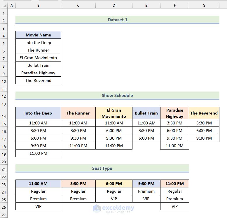
In the following dataset, we have Movie Name, Show Schedule, and Seat Type for some ongoing shows at a cineplex. We’ll create a multi-level hierarchy using this data.
Step 1 – Editing Data Validation Option for Movie Name Column
In the Movie Name column, we need to create a drop-down list from which to select movies.
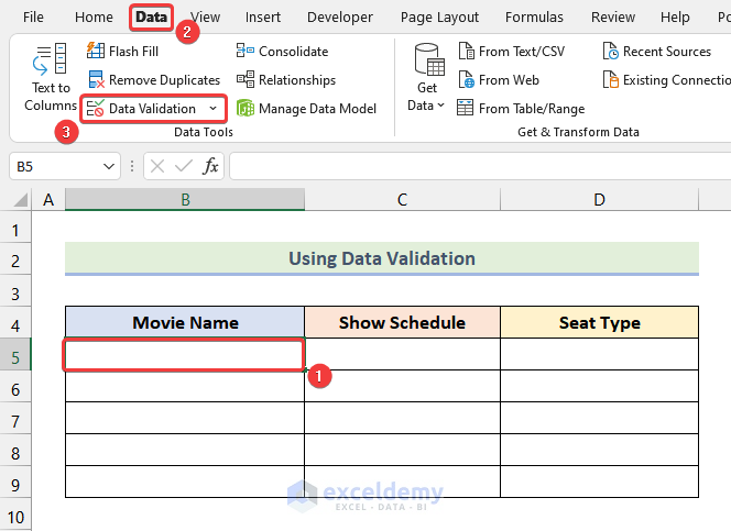
- Select cell B5 under the column Movie Name.
- Go to the Data tab on the Ribbon.
- Click on the Data Validation option from the Data Tools group.
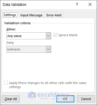
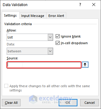
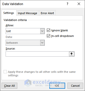
The Data Validation dialog box will open.
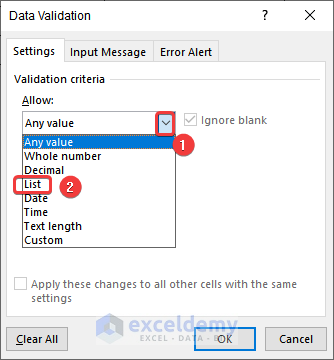
- Click on the drop-down icon as marked in the image below.
- Select List from the drop-down.
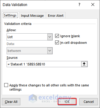
- Click on the Source box and enter the following formula:
='Dataset 1 '!$B$5:$B$10$B$5:$B$10 is the range of the cells in the Movie Name column.
Note: We’ve used absolute cell reference because we want to show the same list of movie names in each cell.
- Click OK.
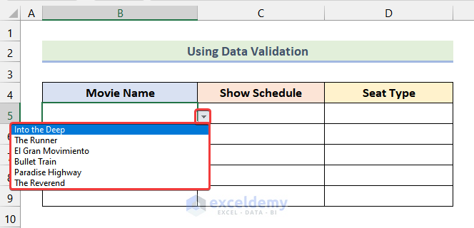
- Click on the drop-down icon beside cell B5 as marked in the following picture.
- From the drop-down list, choose any movie you like.
Step 2 – Pasting Validation Feature in Remaining Cells in Movie Name Column
Now we will use the Paste Special feature of Excel to paste the Data Validation in cell B5 into the other cells of the Movie Name column.
- Select cell B5 and press CTRL + C to copy it.
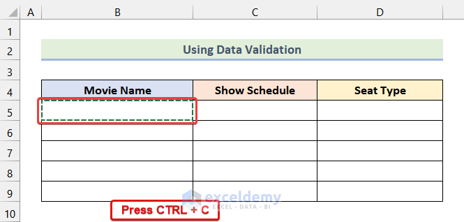
- Select the remaining cells of the column Movie Name.
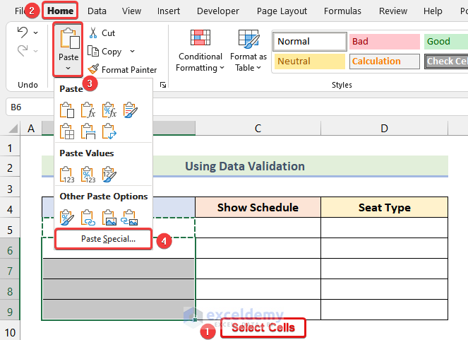
- Go to the Home tab on the Ribbon.
- Click on the Paste option.
- Select Paste Special from the drop-down.
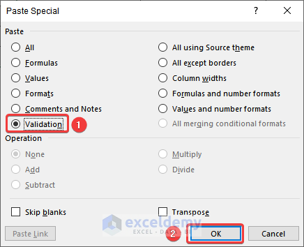
- From the Paste Special dialog box that opens, choose the Validation option.
- Click on OK.
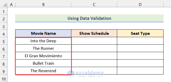
The Data Validation feature will be copied to the selected cells. Choose any of the Movie Names from the drop-down list beside each cell to get an output like in the following image.
Step 3 – Editing Data Validation Option for Show Schedule Column
Now we need to create a drop-down list of screening times in the Show Schedule column based on the selection in the Movie name column. For example, the movie Into the Deep has shows available at 5 different times of the day, but the movie Bullet Train is only available at 3 different times of the day. So, the options that will be available in the Show Schedule column depend on the movie selected in the Movie Name column. To accomplish this, we’ll use the OFFSET function and the MATCH function.
- Select cell C5 and follow the steps in Step 1 to obtain the following output:

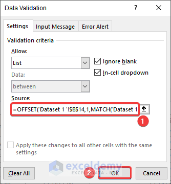
- Enter the following formula in the Source box:
=OFFSET('Dataset 1 '!$B$14,1,MATCH($B5,'Dataset 1 '!$B$14:$G$14,0)-1,5,1)Here, cell $B$14 refers to the header of the Show Schedule of Dataset 1, cell $B5 represents the selected movie under the Movie Name column, and the range $B$14:$G$14 is the array of movie names in Dataset 1.
Formula Breakdown
- MATCH($B5,’Dataset 1 ‘!$B$14:$G$14,0) → returns the position of a lookup value in a row, column, or table.
- $B5 → is the lookup_value argument.
- ‘Dataset 1 ‘!$B$14:$G$14 → is the lookup_array argument.
- 0 → is the match_type argument.
- Output → 1
- OFFSET(‘Dataset 1 ‘!$B$14,1,MATCH($B5,’Dataset 1 ‘!$B$14:$G$14,0)-1,5,1) → becomes OFFSET(‘Dataset 1 ‘!$B$14,1,1-1,5,1)
- ‘Dataset 1 ‘!$B$14 → is the reference argument.
- 1 → is the rows argument.
- 1-1 → is the cols argument.
- 5 → is the height argument.
- 1 → is the width argument.
- Output → {11:00 AM, 3:30 PM, 6:00 PM, 9:30 PM, 11:00 PM}
- Click on OK.
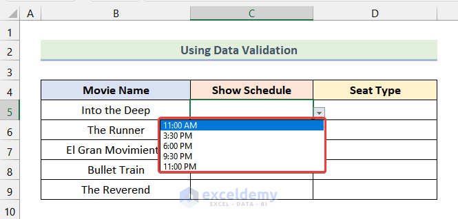
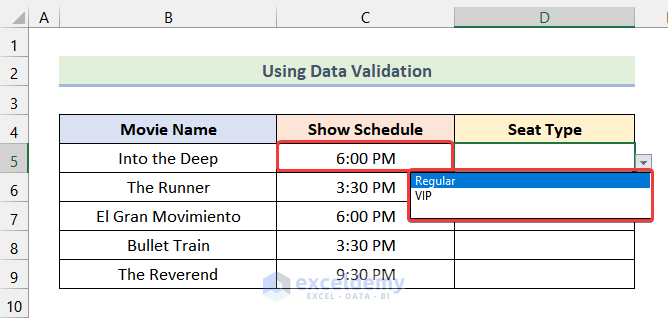
As a result, a drop-down icon will be visible beside cell C5 as shown in the image below.
- Click on it.
The available Show Schedule options for the movie Into the Deep are listed in the drop-down.
Step 4 – Pasting Validation Feature in Remaining Cells in Show Schedule Column
Now we copy the Data Validation properties of cell C5 into the remaining cells by using the Paste Special feature.
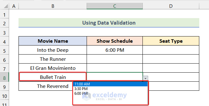
- Select cell C5 and follow the steps in Step 2.
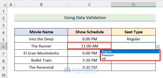
- Choose the movie Bullet Train, and there are only 3 available options for the Show Schedule, just like in our given dataset.
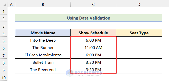
- Choose the Show Schedule for the other movies to get an output like the image below.
Step 5 – Editing Data Validation Option for Seat Type Column
Now we need to create another drop-down list in the Seat Type column based on our selection of the Show Schedule. In the dataset, the Show Schedule options don’t have the same Seat Type. For example, for the show at 11:00 AM, all 3 Seat Types are available, but for the show at 6:00 PM, only the Regular and VIP Seat Types are available. To create this dependent drop-down list, we will again use the OFFSET function and the MATCH function.
- Select cell D5 and follow the steps mentioned in Step 1 to get the following output:
- Enter the following formula in the Source box in the Data Validation dialog box:
=OFFSET('Dataset 1 '!$B$23,1,MATCH($C5,'Dataset 1 '!$B$23:$F$23,0)-1,3,1)Cell $B$23 refers to the header of Seat Type in Dataset 1, cell $C5 represents the selected Show Schedule, and the range $B$23:$F$23 is the array of the Show Schedule in Dataset 1.
Formula Breakdown
- MATCH($C5,’Dataset 1 ‘!$B$23:$F$23,0) → returns the position of a lookup value in a row, column, or table.
- $C5 → is the lookup_value argument.
- ‘Dataset 1 ‘!$B$23:$F$23 → is the lookup_array argument.
- 0 → is the match_type argument.
- Output → 3
- OFFSET(‘Dataset 1 ‘!$B$23,1,MATCH($C5,’Dataset 1 ‘!$B$23:$F$23,0)-1,3,1) → becomes OFFSET(‘Dataset 1 ‘!$B$23,1,3-1,3,1).
- ‘Dataset 1 ‘!$B$23 → is the reference argument.
- 1 → is the rows argument.
- 3-1 → is the cols argument.
- 3 → is the height argument.
- 1 → is the width argument.
- Output → {Regular, VIP}
- Click on OK.
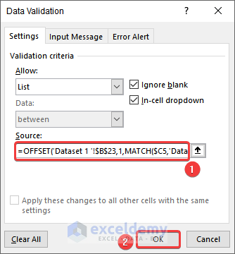
A drop-down icon appears beside cell D5. As the Show Schedule selected is 6:00 PM, the Regular and the VIP options are available in cell D5.
Step 6 – Pasting Validation Feature in Remaining Cells in Seat Type Column
Now copy the Data Validation properties of cell D5 to the other cells of the column Seat Type.
- Select cell D5 and follow the steps in Step 2.
- Click on the drop-down icon beside cell C6. As the Show Schedule selected is 11:00 AM, all 3 Seat Types are available.
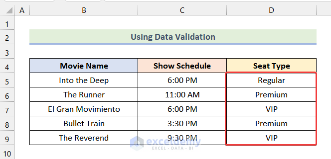
- Similarly, select the Seat Type option for the other cells to get an output like the following picture:
Method 2 – Using Power Pivot
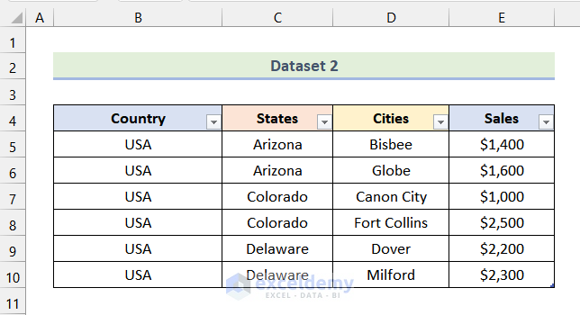
In the following dataset, we have a table of Sales data from different Cities in various States of the USA. We will create a multi-level hierarchy using this table.
Step 1 – Adding the Table to the Power Pivot Window
- If you don’t have the Power Pivot Add-in enabled, then enable it and import data.
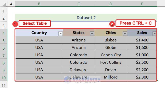
- Select the entire table and press CTRL + C to copy it.
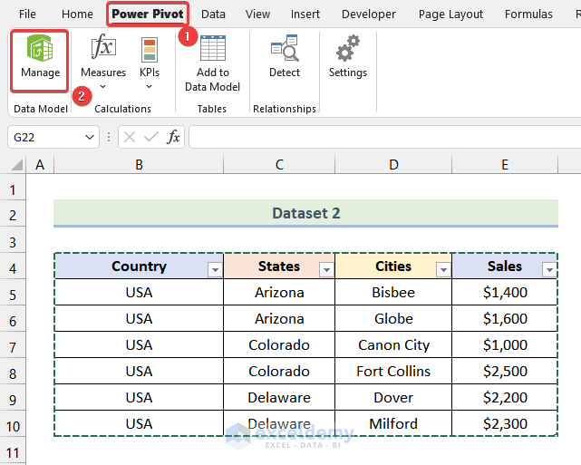
- Go to the Power Pivot tab on the Ribbon.
- Click on the Manage option.
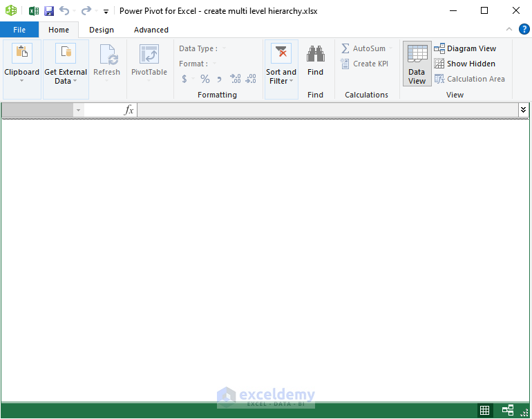
A blank Power Pivot Window will open.
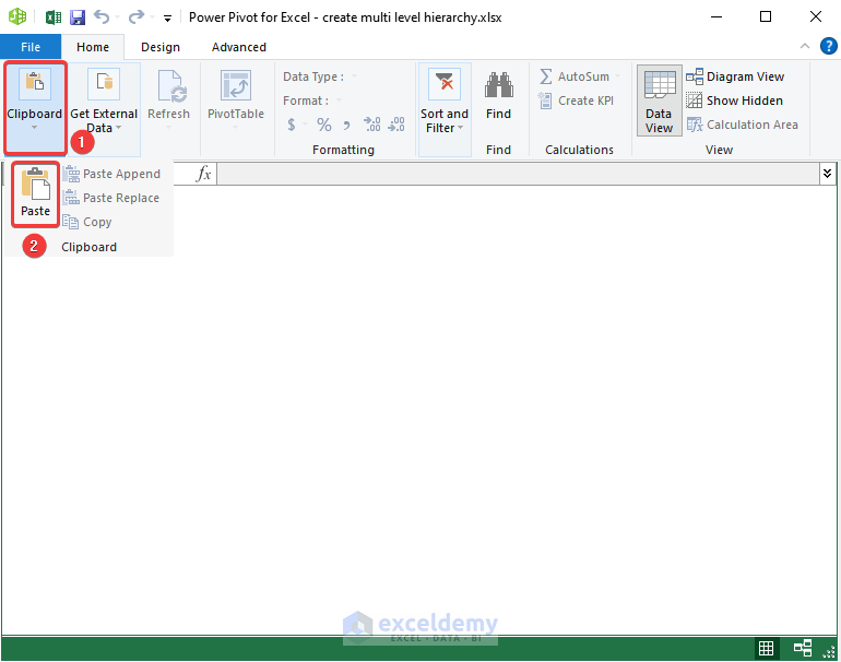
- In the Power Pivot Window, click on the Clipboard option.
- Select the Paste option from the drop-down.
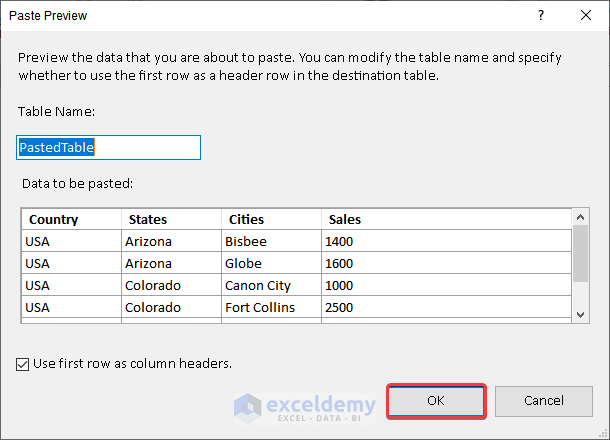
The Paste Preview dialog box will open.
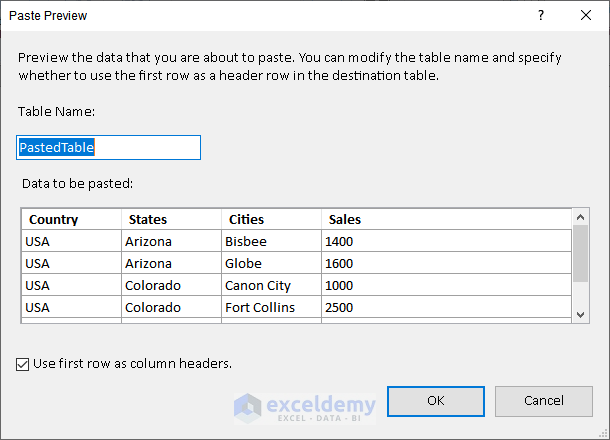
- In the Paste Preview dialog box, click on OK.
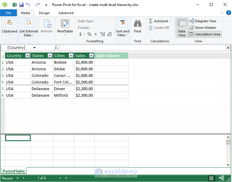
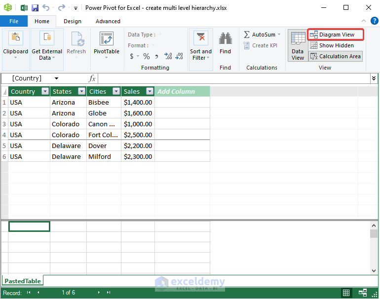
The table will be added to the Power Pivot Window as shown in the following image.
Step 2 – Creating Hierarchy in Diagram View
Now we create a hierarchy that describes the cities under the states and the states under the country.
- Click on the Diagram View option from the View tab of the Power Pivot window.
The Diagram View opens.
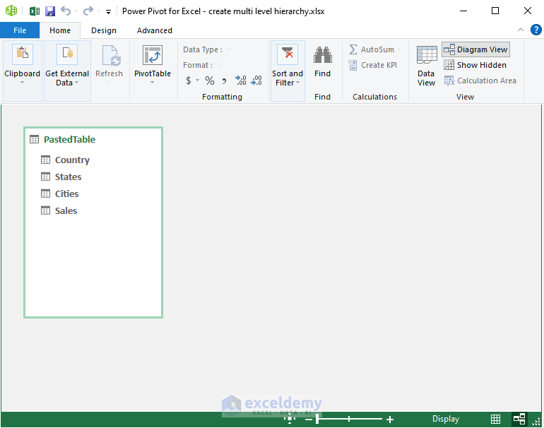
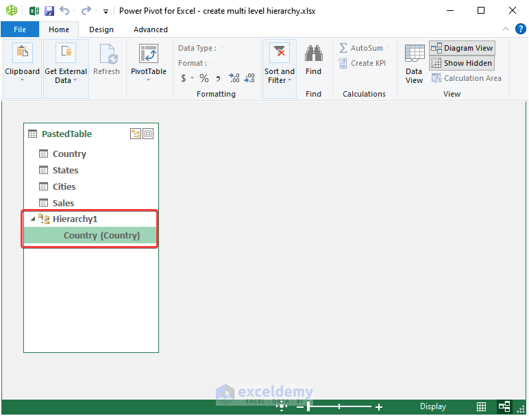
- Click on the marked portion of the image below.
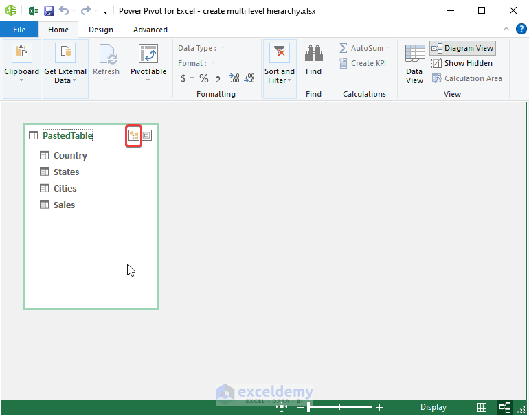
A Hierarchy will be created.
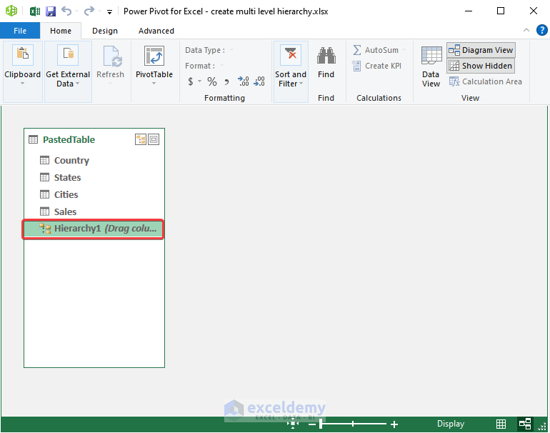
- Drag the column named Country and drop it into the newly created Hierarchy.
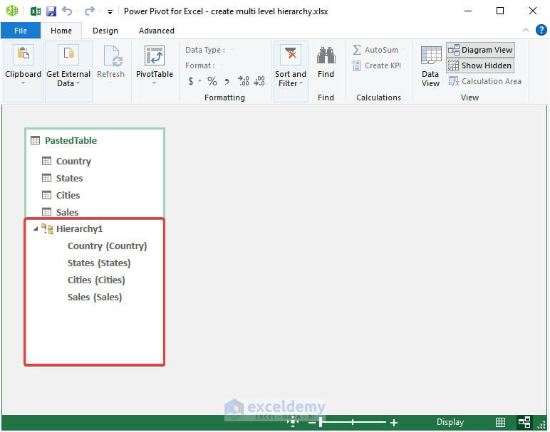
- Similarly, drag and drop the other columns sequentially to get the following output:
Read More: How to Create a Hierarchy of the State City and Zip Code in Excel
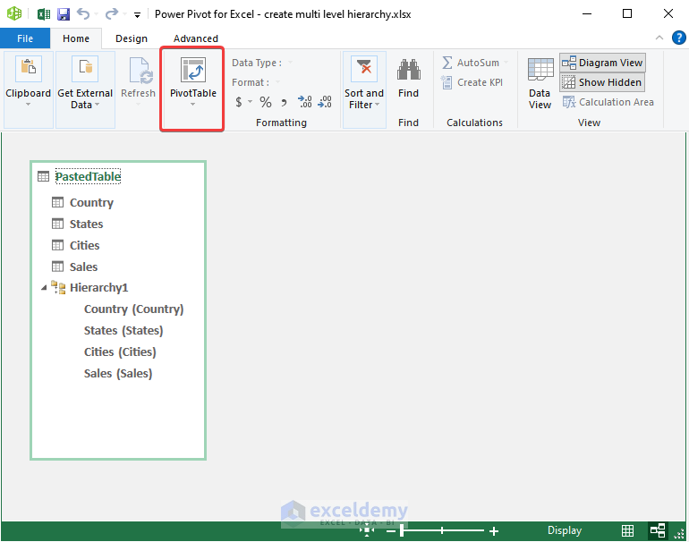
Step 3 – Constructing Pivot Table
- Click on the Pivot Table option.
- In the Create Pivot Table dialog box that opens, click OK.
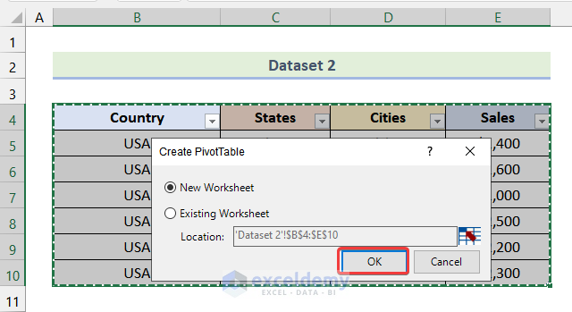
A new worksheet will be created as shown in the following picture.
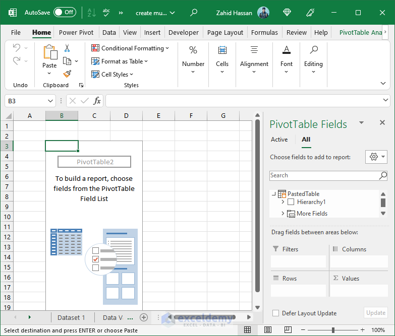
- From the Pivot Table Fields dialog box, drag and drop Hierarchy1 into the Rows section and Sales into the Sum of Values section.
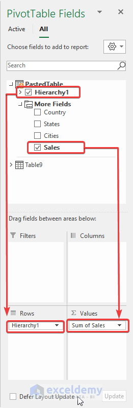
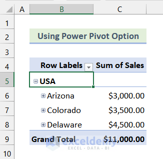
The following Pivot Table will be inserted into the worksheet.
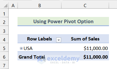
- Click on the + sign as marked in the following picture.
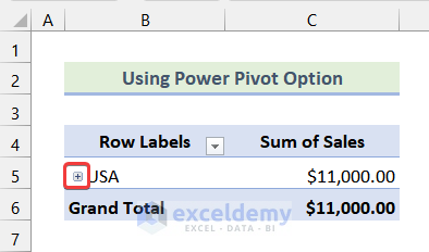
The States, and the Sum of Sales of each State are shown, as in the following image.
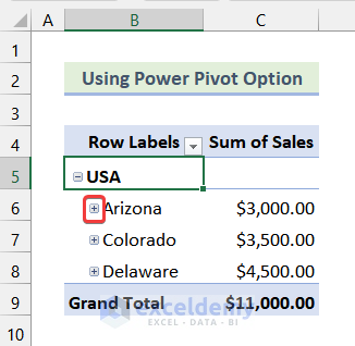
- Again click on the + sign beside the name of the State Arizona.
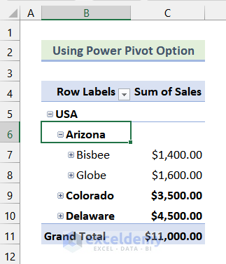
The Cities in the State of Arizona are shown, along with their Sales.
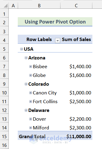
Similarly, by clicking the + icon beside the other States, the following output will be returned.
Read More: How to Create Hierarchy in Excel Pivot Table
Related Articles
- Create Date Hierarchy in Excel Pivot Table
- How to Use SmartArt Hierarchy in Excel
- How to Add Row Hierarchy in Excel
- How to Make Hierarchy Chart in Excel
<< Go Back to Hierarchy in Excel | SmartArt in Excel | Learn Excel
Get FREE Advanced Excel Exercises with Solutions!
