In Excel, the term “hierarchy” has two distinct meanings. The first definition refers to a chart that aids in visualizing a hierarchical structure, such as an organizational chart. Power Pivot hierarchies, on the other hand, let you quickly drill up and down through a list of nested columns in a table.
In this article, we will discuss 3 easy ways to create a hierarchy in Excel. Firstly, we will use the SmartArt feature. Then, we will create a hierarchy in a Pivot Table. Finally, we will illustrate the use of the Power Pivot toolbar to create a hierarchy in Excel.
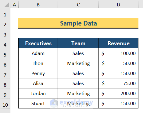
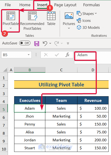
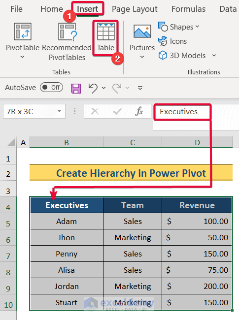
We will use the sample data below to illustrate the methods.
Method 1 – Using the SmartArt Feature to Create Hierarchy in Excel
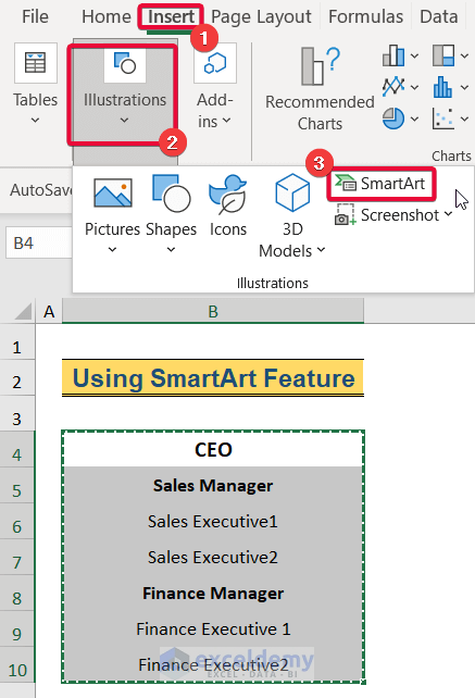
In this method, we will visually represent the hierarchy of an organization using the SmartArt feature.
Steps:
- Copy the entire dataset.
- Go to the Insert tab on the ribbon.
- From the Illustration group, select the SmartArt toolbar.
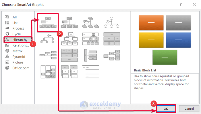
A dialog bar will open.
- Select the Hierarchy option.
- Choose the type of hierarchy graphic you prefer.
- Click OK.
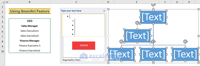
- From the graphic, click on the outward arrow to select a text box.
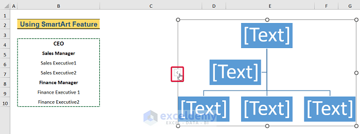
- Keep the cursor on the text box and press Ctrl+A.
All the data in the graphic will be selected.
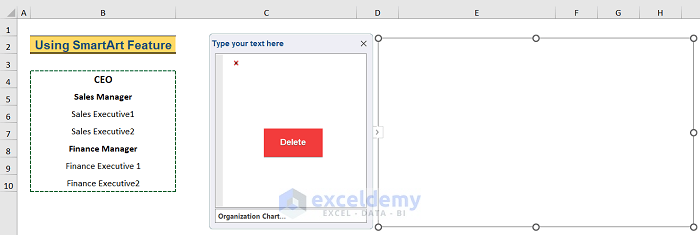
- Press Delete to delete the default data.
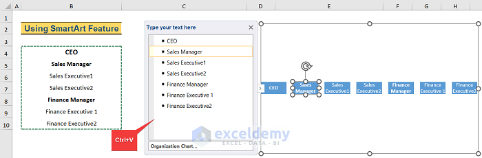
- Keep your cursor on the dialog box and press Ctrl+V.
Our dataset will be pasted into text boxes in the dialog box.
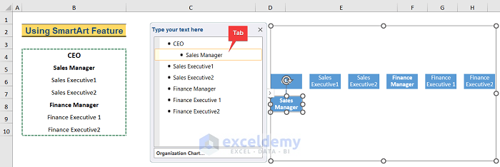
- Choose the Sales Manager option and press Tab once.
Since the Sales Manager reports to the CEO, this new box under the CEO box now illustrates that.
- Select the Sales Executive1 option and press Tab twice.
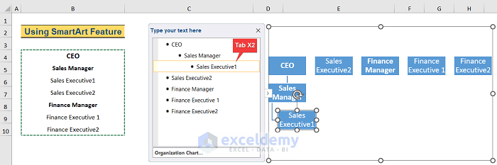
- Repeat the previous two steps to complete the hierarchy illustration.
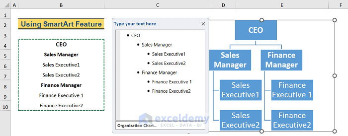
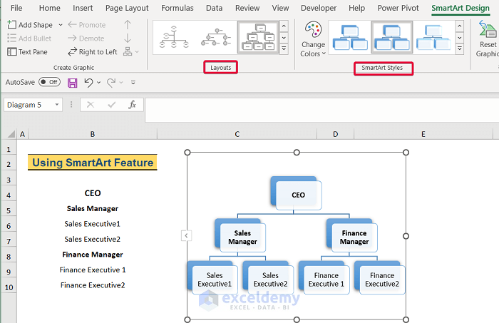
- Format the hierarchy tree by using the Layouts and SmartArt Styles options from the SmartArt Design options.
Our hierarchy chart is complete.
Read More: How to Use SmartArt Hierarchy in Excel
Method 2 – Using a Pivot Table to Create Hierarchy
Now we will use the Pivot Table to create a hierarchy in Excel.
Steps:
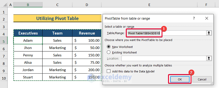
- Select any cell in the dataset.
- Go to the Insert tab on the ribbon.
- Select Pivot Table.
The Pivot Table dialog box will appear.
- In the dialog box, select the range of the dataset as the Table/Range.
- Click OK.
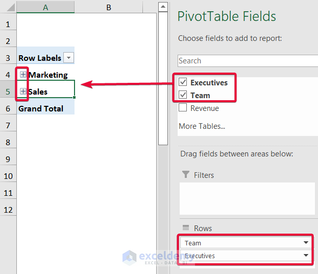
- The PivotTable Fields pane opens in a new worksheet.
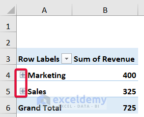
- Select the Executives and Team options from the Pivot Table Fields
The options will be illustrated as Rows in the pivot table.
- Select the Revenue option as Values.
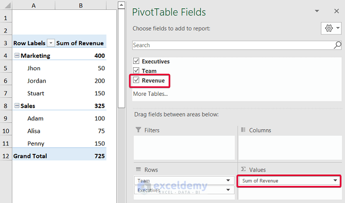
The hierarchy of the different teams is returned.
We can easily show who works in which team/ department, and also their revenue.
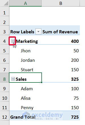
- If you like, minimize the tabs to give a concise view of the pivot table.
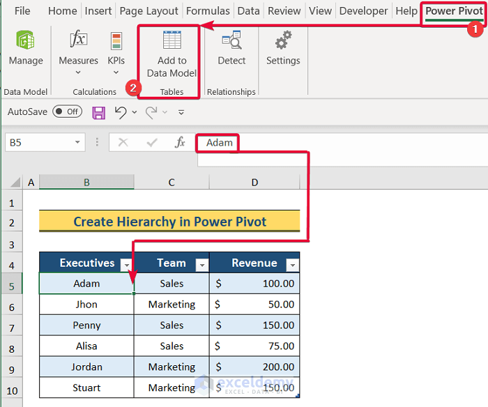
Method 3 – Creating a Hierarchy in Excel Power Pivot
In the final method, we will use the Power Pivot add-in to create a hierarchy. This is a pivot table which allows us to group the data to create a hierarchy.
Steps:
- Select the entire dataset.
- Go to the Insert tab in the ribbon.
- Insert a Table.
- Click OK in the Create Table dialog box.
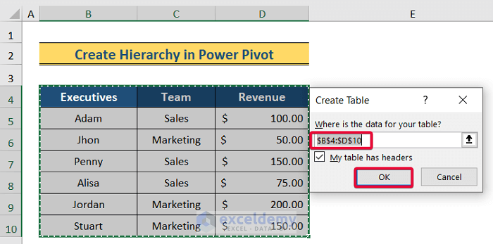
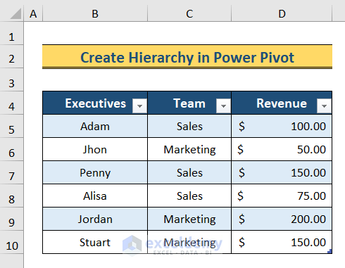
The dataset will be converted into a table.
- Go to the Power Pivot tool bar.
- Select Add to Data Model option.
A new Power Pivot window will open.
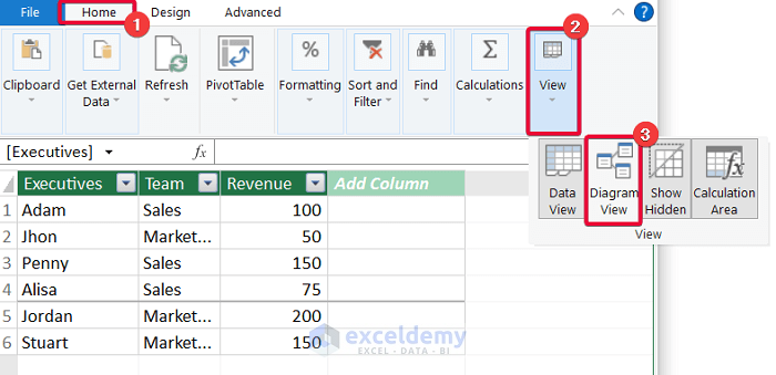
- In the Power Pivot window, go to the Home tab.
- From the View group, select the Diagram View.
The dataset will appear in the diagram view.
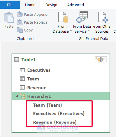
- Right-click after selecting all the options simultaneously.
- From the available options, select Create Hierarchy.
A hierarchy will be created containing all the selected options.
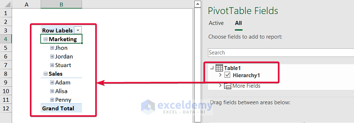
- From the Home tab, select the Pivot Table command.
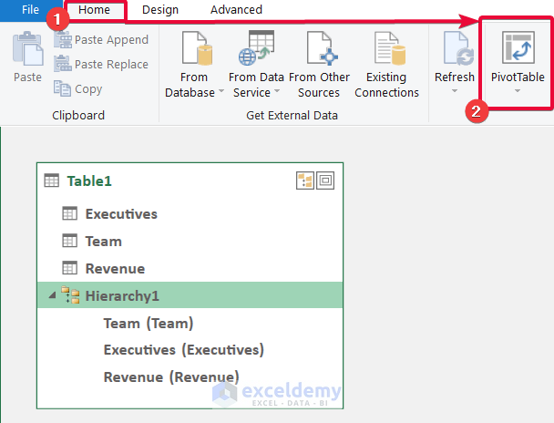
A hierarchy is created.
Download Practice Workbook
Related Articles
- How to Create Multi Level Hierarchy in Excel
- How to Make Hierarchy Chart in Excel
- Create Date Hierarchy in Excel Pivot Table
- How to Create a Hierarchy of the State City and Zip Code in Excel
- How to Add Row Hierarchy in Excel
<< Go Back to Hierarchy in Excel | SmartArt in Excel | Learn Excel
Get FREE Advanced Excel Exercises with Solutions!
